Table of Contents
Market module for agricultural outputs
Overview on the market model
Whereas the outlay of the supply module has not changed fundamentally since the CAPRI project ended in 1999, the market module was completely revised. Even if several independent simulation systems for agricultural world markets are available as OECD’s AgLink, the FAPRI system at the University of Missouri or the WATSIM1) system at Bonn University, it was still considered necessary to have an independent market module for CAPRI.
The CAPRI market module can be characterised as a comparative-static, deterministic, partial, spatial, global equilibrium model for most agricultural primary and some secondary products, in total about 65 commodities, including the young animals that only matter for market clearing in European regions. The list of commodities is chosen to cover as far as possible all products used for food and feed.
It is deterministic as stochastic effects are not covered and partial as it excludes factor (labour and capital) markets, non-agricultural products and some agricultural products as flowers. It is spatial as it includes bilateral trade flows and the related trade policy instruments between the trade blocks in the model.
The term partial equilibrium model or multi-commodity model stands for a class of models written in physical and valued terms. Demand and supply quantities are endogenous in that model type and driven by behavioural functions depending on endogenous prices. Prices in different regions are linked via a price transmission function, which captures e.g. the effect of import tariffs or export subsidies. Prices in different markets (beef meat and pork meat) in any one region are linked via cross-price terms in the behavioural functions. These models do not require an objective function; instead their solution is a fix point to a square system of equations which comprises the same number of endogenous variables as equations.
The CAPRI market module breaks down the world in about 80 countries, each featuring systems of supply, human consumption, feed and processing functions. The regional breakdown is a compromise between full coverage of all individual countries (there are close to 200 UN member countries) and computational data quality considerations. Most countries which a high population number are covered independently, sometimes aggregated with smaller countries. Given the EU focus of CAPRI, agricultural trading partners of the EU are captured in some detail and the regional break down is occasionally updated in view of new trade agreements.
The processing can be differentiated by processing of (a) oilseeds to cakes and oils; (b) biofuel feedstocks to biofuels; © raw milk to dairy products; and (d) any other type of industrial processing. The parameters of all types of behavioural functions are derived from elasticities, borrowed from other studies and modelling systems, and calibrated to projected quantities and prices in the simulation year. The choice of flexible functional forms (normalised quadratic for feed and processing demand as well as for supply, Generalised Leontief Expenditure function for human consumption) and imposition of restrictions (homogeneity of degree zero in prices, symmetry, correct curvature, additivity) on the parameters used ensure regularity as discussed below. Accordingly, the system allows for the calculation of welfare changes for the different agents represented in the market model.
Some of the about 80 countries with behavioural functions (CAPRI set “RMS”) are aggregated for trade policy modelling into in 44 trade blocks or country aggregates (CAPRI set “RM”) with a uniform border protection, and bilateral trade flows are modelled solely between these blocks. Such blocks are EU_WEST, EU_EAST, ‘other Mediterranean’ countries, Uruguay and Paraguay, Bolivia, Chile and Venezuela, and Western Balkan countries. All other countries or country aggregates are identical to one of the 40 trade blocks in the model.
The two EU blocks (EU_WEST, EU_EAST) interact via trade flows with the remaining trade blocks in the model, but each of the EU Member States features an own system of behavioural functions. The prices linkage between the EU Member States and the EU pool is currently simply one of equal relative changes, not at least ease the analysis of results. If regional competitiveness and hence net exports change significantly it may be expected (and has been observed in Hungary since 2004) that prices in ‘surplus’ regions would decrease relative to the EU average, contrary to the assumption of proportional linkage. Alternative specifications have been analysed in the context of the CAPRI-RD project and an option of a flexible definition of EU subaggregates is currently the topic of an ongoing project.
The current break down of the CAPRI market model can be found at http://www.capri-model.org/dokuwiki/doku.php?id=capri:concept:regMarket.
The market model in its current layout comprises about 70.000 endogenous variables and the identical number of equations.
Policy instruments in the market module include (bi)lateral ad-valorem and specific tariffs and, possibly, Producer/Consumer Subsidy Equivalent price wedges (PSE/CSE) where no current data is entered. However, negative entries on the “PSEi” position (for indirect support) have been used in several appications to reflect a global carbon price. Tariff Rate Quotas (TRQs), billaterally allocation or globally open are integrated in the modelling system, as are intervention stock changes and subsidised exports under WTO commitment restrictions for the EU. Subsidies to agricultural producers in the EU are not covered in the market model, but integrated in a very detailed manner in the supply model. For the EU, flexible tariffs for cereals and the minimum import price regime for fruits & vegetables are introduced. Flexible tariffs related to minimum import prices are also present for Switzerland.
The approach of the CAPRI market module
Multi-commodity models are as already mentioned above a widespread type of agricultural sector models. There are two types of such models, with a somewhat different history. The first type could be labelled ‘template models’, and its first example is Swopsim. Template models use structurally identical equations for each product and region, so that differences between markets are expressed in parameters. Typically, these parameters are either based on literature research, borrowed from other models or simply set by the researcher, and are friendly termed as being ‘synthetic’. Domestic policies in template models are typically expressed by price wedges between market and producer respectively consumer prices, often using the PSE/CSE concept of the OECD. Whereas template models applied in the beginning rather simple functional forms (i.e, constant elasticity double-logs in Swopsim or WATSIM), since some years flexible functional forms are in vogue, often combined with a calibration algorithm which ensures that the parameter sets are in line with microeconomic theory. The flexible functional forms combined with the calibration algorithm allow for a set of parameters with identical point elasticities to any observed theory consistent behaviour which at the same time recovers quantities at one point of observed prices and income. Ensuring that parameters are in line with profit respectively utility maximisation allows for a welfare analysis of results.
Even if using a different methodology (explicit technology, inclusion of factor markets etc.), it should be mentioned that Computable General Equilibrium models are template models as well in the sense that they use an identical equation structure for all products and regions. Equally, they are in line with microeconomic theory.
The second type of model is older and did emerge from econometrically estimated single-market models linked together, the most prominent example being the AGLink-COSIMO modelling system. The obvious advantages of that approach are firstly the flexibility to use any functional relation allowing for a good fit ex-post, secondly that the econometrically estimated parameters are rooted in observed behaviour, and thirdly, that the functional form used in simulations is identically to the one used in parameter estimation. The downside is the fact that parameters are typically not estimated subject to regularity conditions and will likely violate some conditions from micro-theory. Consequently, these models are typically not used for welfare analysis. Examples of such models are AGLink-COSIMO at the OECD_FAO, the FAPRI set of market models, or the set of models emerging from AgMemod. However, AGLink-COSIMO is currently in the process to move closer to a template model.
The CAPRI market module is a template model using flexible functional forms. The reason is obvious: it is simply impossible to estimate the behavioural equations for about 65 products and 80 countries or country blocks worldwide with the resources available to the CAPRI team. Instead, the template approach ensures that the same reasoning is applied across the board, and the flexible functional forms allow for capturing to a large degree region and product specificities. As such, the results from econometric analysis or even complete parameters sets from other models could be mapped into the CAPRI market model.
Behavioural equations for supply, feed demand and land markets
The definition of the market model can be found in ‘arm\market_model.gms’
Agricultural supply
Supply for each agricultural output i and region r (EU Member States or regional aggregate) is modelled by a supply function derived from a normalised quadratic profit function via the envelope theorem. Supply depends on producer prices v_prodPrice normalised with a price index. The price index relates to all those goods – either inputs or outputs – which are not explicitly modelled in the system:
\begin{equation} v\_prodQuant_{i,r} = as_{i,r}+ \sum_j bs_{i,j,r} \frac{v\_prodPrice_{j,r}}{p_{index,r}} \end{equation}
Supply curves for the EU Member States, Norway, Turkey, Western Balkans are calibrated in each iteration to the last output price vector used in the supply model and the aggregated supply results at Member State level, by shifting the constant terms as. The slope terms bs which capture own and cross-price effects are set in line with profit maximisation, as discussed below. The calibration of the price dependent parameters bs is discussed below.
For the countries which matching regional models on the supply side, the bs parameters are derived directly from the costs function terms and elements of the constraints matrix (see Chapter 4.3 
Land supply and demand
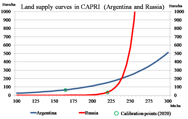
The reader should note that land is one of the products in the above system which is an input into agriculture. A land supply curve defines the demand side of the land balance which together with the land demand according to the equation above define the land rent clearing the balance. Equally, the price for feed energy is an input price entering the equations.
\begin{align} \begin{split} v\_prodQuant_{r,"Land"} = \; & p\_cnstLandSpply_r \\ &+ p\_cnstLandElas_r \; log(v\_prodPrice_{r,"Land"}) \end{split} \end{align}
Figure 18: Land supply curve examples
In order to parameterize the land demand function, information about yield and supply elasticities is used. The marginal reaction of land to a marginal change in one of the prices is defined as the total supply effect minus the yield effect:
\begin{equation} \frac {dLand}{dp_i} = \sum_j \frac {dQ_j}{dp_i} 1/yield_j -ela_i \frac {Q_i}{p_i} 1/yield_i \end{equation}
where Q denotes quantities and p prices. The calibration requires prices for land which is set to 0.3 of the crop revenues. For fodder area demand from animals it was set lower (cp. page 56 in Golub et.al. 2006). The summation term over all products j defines the “land demand change” if the price i changes. The quantity change of each product j is translated into a land demand change based on its yield. The reciprocal of the yield can be interpreted as the land demand per unit produced.
The last term translates first the yield elasticity (an endogenous variable) into a marginal quantity effect and, then again, based on the yield, in a changed land demand. The land demand change is subtracted as the land demand for product i per unit decreases if yields increase due to a positive own price yield elasticity. This formulation assumes, as conventionally done in multi-commodity models, that cross-price yield effects are zero.
The CAPRI market model does not handle explicitly non-tradable crop outputs such as grass, silage or fodder maize. However, the land demand for these products is also taken into account in order to allow closing an overall land balance. This is achieved by deriving per unit land demands for animal products.
The link to land supply is straightforward: if the land supply curve is known, a market balance equilibrates the simulated land demand based on the behavioral equation derived from the NQ profit function with that land supply curve. The land price is the equation multiplier attached to the land market clearing equation. If the land supply curve collapses to a constant, any output price induced change in land demand is leveled out by a change in the land price. That solution is equivalent to the behavior of programming model with a fix land endowment.
If the market balance equation is dropped and the land price fixed, totally elastic land supply to agriculture is assumed. This assumption should be of little empirical value as agriculture is typically the major demander for land suitable to agriculture. The current solution incorporates a land supply curve with exogenous given elasticities (similar to Tabeau et.al. 2006). The parameterization of the land supply curve is currently chosen similar to the land elasticities e.g. reported in GTAP (Ahmed et al. 2008). Generally, land supply is rather inelastic so that price increase of agricultural commodities rather increases land prices and not so much land use.
Although the profit function approach does not allocate areas to individual crops, it captures in a dual formulation how product and land price changes impact on total agricultural land use. The estimated yield elasticity may be used however to derive an allocation which is consistent with the assumptions used during parameter calibration. Basically, for each crop product, the yield elasticity is used to derive from the simulated quantity change the implied land change. The resulting land demands are then scaled to match the simulated change in total land. This allocation is currently active at solution time (with explicit equations) in the “trunk” version of CAPRI but not yet in all branches (in particular not in the “star2.4” version underlying the CAPRI Training 2019).
Feed demand
The system for feed demand for countries not covered by the supply part is structured identically to the supply system. However, not producer prices, but raw product prices v_arm1Price determined by the Armington top level aggregator drive feed demand v_feedQuant, combined with changes in the supply of animal products weighed with feed use factors w:
\begin{equation} v\_feedQuant_{i,r} = \left( af_{i,r} + \sum_j bf_{i,j,r} \frac {v\_arm1Prices_{j,r}} {p_{index,r}} \right) \end{equation}
One of the prices in the equations above is the price for feed energy which is conceptually the output sold by the feed producing industry where products used for feed are its input. A balance between feed energy demanded, derived from the supply quantities and feed energy need for tradeables per unit produced and feed energy delivered from current feed demand quantities drives the price for feed energy:
\begin{equation} \sum_i v\_feedQuant_{i,r} \; p\_calContent_r = \sum_iv\_prodQuant_{i,r} \; pv\_feedConv_{i,r} \end{equation}
For countries which matching modules on the supply side, a different system is set-up. In the supply part, individual commodities are aggregated to categories as cereals. The composition of these aggregates is determined by a CES function, whereas total demand for each category depends on the average price aggregated from the ingredients.
As for supply, feed demand for the aggregate EU Member States, Norway, Turkey and Western Balcans, are calibrated in each iteration to the last output price vector used in the supply model and the aggregated feed demand at Member State level.
The disadvantage of the behavioural functions above is the fact that they might generate non-positive values. That situation might be interpreted as a combination of prices where the marginal costs exceed marginal revenues. Accordingly, a fudging function is applied for supply, feed and (see below) processing demand which ensures strictly positive quantities. That fudging function is highly non-linear, and therefore only switched on on demand.
Behavioural equations for final demand
The final demand functions are based on the following family of indirect utility functions depending on consumer prices cpri and per capita income y2) where G and F are functions of degree zero in prices (RYAN & WALES 1996) which will be defined below3):
\begin{equation} U(cpri,y) = \frac {-G} {y-F} \end{equation}
Using Roy’s identity, the following per capita Marshallian demands PerCap are derived:
\begin{equation} PerCap_i = F_i+ \frac {G_i} {G} (y-F) \end{equation}
where the \(F_i\) and \(G_i\) are the first derivative of F and G versus own prices. The function F is defined as follows:
\begin{equation} F_r = \sum_i d_i \; cpri_i \end{equation}
where the \(d_i\) have a similar role as constant terms in the Marshallian demands and can be interpreted as ‘minimum commitment levels’ or consumption quantities independent of prices and income. The term in brackets in the per capita demands in Equation 122 
\begin{equation} G = \sum_i \sum_j bd_{ij} \sqrt {cpri_i \; cpri_j} \end{equation}
with the derivative of G versus the own price is labelled \(G_i\) and defined as:
\begin{equation} G_j = \sum_i bd_{ij} \sqrt {cpri_i / cpri_j} \end{equation}
Symmetry is guaranteed by a symmetric bd matrix describing the price dependent terms, correct curvature by non-negative the off-diagonal elements of bd, adding up is automatically given, as Euler’s Law for a homogenous function of degree one \( \left ( a(x) = \sum_i \frac{\partial a(x)}{\partial x_i}x_i \right ) \) , leads to:
\begin{align} \begin{split} \sum_i PerCap_i \; cpri_i &= \frac{\sum_i G_icpri_i}{G}(y-F)+ \sum_i d_icpri_i\\ &= \frac{ G}{G} (y-F)+ F = \; y \end{split} \end{align}
and homogeneity is guaranteed by the functional forms as well. The expenditure function follows from rearranging Equation 121 
\begin{equation} y = e(U,cpri)=F- \frac{G}{U} \end{equation}
The function is flexible to reflect all conceivable own price and expenditure elasticities but the non-negativity imposed on the off-diagonal elements ensuring excludes Hicksian complementarity, a restriction not deemed important in the light of the product list covered. Note that concavity of e is given if G is concave, as U < 0 and F is linear. Concavity of G in turn follows from nonnegative off-diagonal \(bd_{ij}\) without further restrictions, because G is then a sum of concave elementary functions \(bd_{i,j} (cpri_i cpri_j)^{0.5}\) with the linear terms on the diagonal being both concave and convex regardless of signs of \(bd_{ii}\).
Human consumption hcom is simply the sum of population pop multiplied with the per capita demands:
\begin{equation} hcom_{i,r} = pop_r \; PerCap_{i,r} \end{equation}
Behavioural equations for the processing industry
Processing demand for oilseeds is modelled by using behavioural functions derived from a normalised quadratic profit function under the assumption of a fixed I/O relation between seeds, cakes and oils. Consequently, the processing demand proc depends on processing margins procMarg which are differences between the value of the outputs (oil and cake) per unit of oilseed processed and the value of the oilseed inputted:
\begin{equation} v\_procMarg_{i,r} = ac_{i,r}+ \sum_j bc_{i,j,r} \frac{v\_procMarg_{j,r}}{p_{index,r}} \end{equation}
The processing margins are replaced by producer prices times -1 for all products besides oilseed. For the latter, the processing margin is defined from the producer prices v_prodPrice for the cakes and oils time the respective crushing coefficients minus the buying prices (average of domestically sold and imported quantities) v_arm1Price:

\begin{align} \begin{split} v\_prodMarg_{seed,r} = &-v\_arm1Price_{seed,r} \\ & +v\_prodPrice_{seed \rightarrow cak,r} v\_procYield_{cak,r} \\ & +v\_prodPrice_{seed \rightarrow oil,r} v\_procYield_{oild,r} \\ \end{split} \end{align}
Finally, output of oils and cakes supply depends on the processed quantities proc of the oilseeds and the crushing coefficients:

\begin{align} \begin{split} supply_{cake,r} = proc_{seed,r} v\_procYield_{cak,r} \\ supply_{oil,r} = proc_{seed,r} v\_procYield_{oil,r} \\ \end{split} \end{align}
The processing yields in the base year are defined as:
\begin{equation} v\_procYield_{cak,r} = \frac{v\_prodQuant_{seed \rightarrow cak,r}^{bas}}{v\_prodQuant_{seed,r}^{bas}} \end{equation}
The processing yields are however not fixed during simulation, but depend on a CES function: the share of oil increases very slightly if the oil price increases compared to the cake price, and vice versa.
Special attention is given to the processing stage of dairy products. First of all, balancing equations for fat and protein ensure that the processed products use up exactly the amount of fat and protein comprised in the raw milk. The fat and protein content of raw milk cont and milk products mlk is based on statistical and engineering information, and kept constant at calibrated base year levels.
\begin{equation} v\_prodQuant_{"milk",r}cont_{"milk",fp} = \sum_{mlk} v\_prodQuant_{mlk,r}cont_{mlk,fp} \end{equation}
Production of processed dairy products is based on a normalised quadratic function driven by the difference between the dairy product’s market price and the value of its fat and protein content.
\begin{align} \begin{split} v\_prodQuant_{mlk,r} = &am_{mlk,r} \\ &+ \sum_j bm_{mlk,j,r} \frac {v\_prodPrice_j-cont_{j,"fat"}pFatProt_{fat,r}-cont_{j,"prot"}pFatProt_{prot,r}}{p_{index,r}} \end{split} \end{align}
And lastly, prices of raw milk are derived from its fat and protein content valued with fat and protein prices and a processing margin.
Trade flows and the Armington assumption
The Armington assumption drives the composition of demand from domestic sales and the different import origins depending on price relations and thus determines bilateral trade flows (Armington 1969). The Armington assumption is frequently used in that context, and e.g. applied in most Computable General Equilibrium models to describe the substitution between domestic sales and imports.
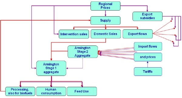
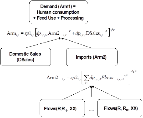
The underlying reasoning is that of a two-stage demand system. At the upper level, demand for products such as wheat, pork etc. is determined as a function of prices and income – see above. These prices are a weighted average of products from different regional origins. At the lower level, the composition of demand per product i in region r stemming from different origins r1 is determined based on a CES utility function:
\begin{equation} U_{i,r} = \alpha_{i,r} \left [\sum_{r1} \delta_{i,r,r1}M_{i,r,r1}^{1/\rho_{r,i}} \right]^{1/\rho_{r,i}} \end{equation}
where U denotes utility in region r and for product i due to consumption of the import quantities M stemming from the different origins r1. If r is equal r1, M denotes domestic sales. \(\delta\) are the share parameters, \(\alpha\) is called the shift-parameter, and \(\rho\) is a parameter linked to the substitution elasticity \( \sigma = 1/(1+\rho)\). Deriving the first order conditions for utility maximisation under budget constraints leads after lengthy re-arrangements to the following relation between imported quantity \(M_{i,r,r1}\), utility \(U_{i,r}\) (quantity aggregator), import price \(P_{i,r,r1}\), and the aggregate import price \(P_{i,r}\):
\begin{equation} M_{i,r,r1} = U_{i,r} \delta_{i,r,r1}^{\sigma_{r,i}} \left [ \frac{P_{i,r}}{P_{i,r,r1}} \right]^{\sigma_{r,i}} \quad \text {(importShares_)} \end{equation}
As seen from the equation, imports from region r1 will increase if its competitiveness increases – either because of a lower price in r1 or a higher average import price. The resulting changes in the compositions of imports increase with the size of the related share parameter \(\delta_{i,r,r1}\) and with the size of the substitution elasticity. The CES utility function is rather restrictive as it has solely one parameter \(\delta\) per import flow. The substitution elasticity \(1/(1+\rho)\) is set exogenously, see below. The \(\delta\) parameters are determined when calibrating the model to known import flows, whereas \(\alpha\) is used to meet the known quantities in the calibration point (and effectively is in the \(\delta\) parameters in the implementation in the code).
The model comprises a two stage Armington system (see below): on the top level, the composition of total demand from imports and domestic sales is determined, as a function of the relation between the domestic price and the average import price. The lower stage determines the import shares from different origins and defines the average import price. This also means that the implementation in the code has to distinguish between a top and lower level level quantity (or price) aggregate. The substitution elasticity on the top level stage is smaller than for the second one, i.e. we assume that consumers will be less responsive regarding substitution between domestic and imported goods compared to changes in between imported goods.
The following table shows the substitution elasticities used for the different product groups. Compared to most other studies, we opted for a rather elastic substitution between products from different origins, as agricultural products are generally more uniform then aggregated product groups, as they can be found e.g. in CGE models.
Table 28: Substitution elasticities for the Armington CES utility aggregators4)
| Product (group) | Substitution elasticity between domestic sales and imports | Substitution elasticity between import flows |
|---|---|---|
| Cheese, fresh milk products | 2 | 4 |
| Other vegetables | 1.5 | 1.5 |
| Other fruits | 3 | 3 |
| Sugar | 12 | 12 |
| All other products | 8 | 10 |
There are some specific settings, such as a value of 2 for rice and the EU15, 2.5 respectively 5 for Japan to account for its specific tariff system, as well as some lower values for EU’s Mediterrean partner countries.
Figure 19: Two-stage Armington System
Soruce: Capri Modelling System
The above “primal” formulation of the Armington approach in terms of quantity aggregators turned out numerically less stable in the implementaiotn than the dual representation in terms of price aggregators. The Armington approach suffers from two important shortcomings. First of all, a calibration to a zero flow is impossible so that only observed import flows react to policy changes while all others are fixed at zero level. For most simulation runs, that shortcoming should not be serious. If it is relevant, it may be overcome using the modified Armington approach as explained in Section Price linkages.
Secondly, the Armington aggregator defines a utility aggregate and not a physical quantity. That second problem is healed by re-correcting in the post model part to physical quantities. Little empirical work can be found regarding the estimation of the functional parameters of Armington systems. Hence, substitution elasticities were chosen as to reflect product properties as shown above.
Market clearing conditions
All quantities in the model are measured in thousand metric tons. The quantity balances for the trade blocks first state that production must be equal to domestic sales plus export flows plus changes in intervention stocks:
\begin{align} \begin{split} v\_domSales_{i,r} = &v\_prodQuant_{i,r} \\ &-v\_expQuant_{i,r} \quad \quad \text {(SupBalM_)}\\ &+v\_intervStockChange_{i,r} \\ \end{split} \end{align}
Further on, imports and exports are defined from bilateral trade flows as:
\begin{equation} v\_impQuant_{i,r} = \sum_{r\ne r1} v\_tradeFlows_{i,r,r1} \quad\text{(impQuant_)} \end{equation}
\begin{equation} v\_expQuant_{i,r} = \sum_{r\ne r1} v\_tradeFlows_{i,r,r1} \quad\text{(expQuant_)} \end{equation}
Finally, the Armington first stage aggregate - arm1, shown in the diagram above, is equal to the domestic consumption elements feed, human consumption and processing:
\begin{align} \begin{split} v\_arm1Quant_{i,r} = &v\_feedQuant_{i,r} \\ &+v\_consQuant_{i,r} \\ &+v\_procQuant_{i,r} \quad \quad \text {(armBall_)}\\ &+v\_biofprocQuant_{i,r} \end{split} \end{align}
The reader should note that for those trade blocks comprising several countries such as the EU, the right hand side quantities are an aggregate over individual countries.
Price linkages
All prices in model are expressed as € per metric ton. Import prices - \(impp_{i,r,r1}\) from region r1 into region r of product i are determined from market prices v_marketPrice times a possible exogenous change in exchange rates compared to the baseline minus export subsidies expsub plus bi-lateral transport costs aking into account bilateral ad valorem (v_tarAdval) and specific (v_tarSpec) tariffs respectively flexible levies (DiffLevies):
\begin{align} \begin{split} impp_{i,r,r1} = & \left [ \begin{matrix} v\_marketPrice_{i,r1}\, p\_exchgRateChangeFaktor_{r,r1} \\ -expsub_{i,r1}+ v\_transpCost_{i,r,r1} \\ \end{matrix} \right ] \\ &(1+v\_tarAdVal_{i,r,r1}/100)+v\_tarSpec_{i,r,r1}+DiffLevies_{i,r,r1} \end{split} \end{align}
Bilateral tariffs may be endogenous variables if they are determined by a tariff rate quota (TRQ), see below. Equally, export subsidies are endogenous variables.
Producer prices are derived from market prices formally using direct and indirect PSEs price wedges – albeit these are all zero at currently -, except for EU_WEST, EU_EAST and Bulgaria and Romania. The reader is reminded that for the EU, the supply model includes a rather detailed description of the different premium schemes of the CAP, so that the EU premiums need not to be modelled as price wedges in the market part. In cases where several countries are comprised in a trade block, the market price refers to the trade block. The “Pmrg” is a factor which is defined such that observed producer prices are recovered.
\begin{equation} v\_prodPrice_{i,r} = [ v\_marketPrice_{i,r} + PSEd_{i,r} + PSEi_{i,r} ] Pmrg_{i,r} \end{equation}
The reader is reminded that currently, the PSE data are not introduced in the system with two exceptions: carbon price scenarios involve negative PSEi amounts and Swiss agricultural policies are involving land subsidies entered.
The average prices of imports derived from the Armington second stage aggregate are labelled v_arm2Price:
\begin{equation} v\_arm2P_{i,r} = \left [ \sum_{r1} \delta_{i,r,r1}^{\sigma_{2,r,i}}v\_impP_{i,r,r1}^{1-\sigma_{2,r,i}}\right] ^{1/(1-\sigma_{2,r,i})} \quad \text {(arm2PriceAgg_)} \end{equation}
Similarly, the average prices for goods consumed domestically - arm1p are a weighted average of the domestic market price \(v_marketPrice_{i,r}\) and the average import price \(v_arm2P_{i,r}\):
\begin{equation} v\_arm1P_{i,r} = \left [ \sum_{r1} \delta_{i,m}^{\sigma_{r,i}}P_{i,r,D}^{1-\sigma_{r,i}}\right] ^{1/(1-\sigma_{r,i})} \end{equation}
where \(D \in \{M,S\}, P_{i,r,M} = v\_arm2P_{i,r} \) and \(P_{i,r,S} = v\_marketPrice_{i,r} \). Consumer prices - v_consPrice are derived from the composite good price index v_arm1Price taken into account policy introduced price wedges as direct and indirect consumer subsidy equivalents (currently not available) plus a fix margin covering transport, processing and all other marketing costs:
\begin{equation} v\_consPrice_{i,r} = v\_arm1Price_{i,r} - CSEd_{i,r}-CSEi_{i,r}+cmrg_{i,r} \end{equation}
Unit value exports net of border protection are defined as average market prices in the export destination minus tariffs as:
\begin{align} \begin{split} v\_unitValueExports_{i,r} =\frac{\sum_{r1 \ne r} (pmrk_{i,r1}-tariffs_{i,r,r1})/(1-tariffa_{i,r,r1}) v\_tradeFlows_{i,r,r1}}{v\_nonDoubleZeroEports_{i,r}} \end{split} \end{align}
The unit values exports are used to define the per unit export subsidies - expsub as shown in the equation below. The parameter cexps is used to line up the market equation with the subsidies observed ex-post. Per unit export subsidies hence increase, if market prices pmrk increase or export unit values uvae drop, or if the share of subsidised exports exps on total exports increase. How the amount of subsidised exports is determined is discussed below.
\begin{equation} expsub_{i,r} = \frac{exps_{i,r}}{exports_{i,r}}(pmrk_{i,r}-uvae_{i,r}+cexps_{i,r}) \end{equation}
The Armington aggregator functions are already shown in the diagram above. The compositions inside of the Armington composite goods can be derived from first order conditions of utility maximisation under budget constraints and lead to the following conditions:

Similarly, relations between import shares are determined by:
\begin{equation} \frac{v\_tradeFlows_{i,r,r1}}{v\_tradeFlows_{i,r,r2}}= \left( \frac{dp_{i,r,r1}}{dp_{i,r,r2}} \frac {impp_{i,r,r2}}{impp_{i,r,r1}} \right )^{\frac{1}{1+\phi_2}} \end{equation}
Modified Armington import demand system
The standard Armington import demand system in CAPRI has been extended in a study on behalf of JRC-IPTS (154208.X1) in order to tackle the zero trade-flow issue. The zero-trade issue concerns the inability to model emerging bilateral trade relations in the current version of the CAPRI model. Emerging trade flows in this context are those that are zero in the corresponding baseline, but that are expected to be significant under specific scenario assumptions (e.g. trade liberalization scenarios removing prohibitive trade barriers).
Methodology
The traditional approach in Armington trade models applies the CES functional form in a nested import demand structure. The CES functional form, however, cannot be calibrated against zero observations. The easiest illustration probably is to recall the import demand function and import price aggregator from above. In case of zero flows the share parameter \(\delta_{i,r}\) becomes zero and thus the trade flows will have no contribution to the price index. Furthermore, the import demand equation cannot assign zero values when prices, share parameters, the quantity aggregate and the substitution elasticity are all positive.
To overcome the inability of calibrating the import-demand system to zero observations the approach of Witzke et al. (2005) has been implemented in CAPRI. This modifies the standard CES form by shifting them with an additional commitment term. That additional (commitment) term requires not only the observed price/quantity points but additional information. The additional information in this case covers expected imports under a hypothetical set of relative import prices that differ from the observed ones. The approach is illustrated in the simple two-goods case, where good 2 is not imported in the calibration point, but is expected to be positive if its relative price to good 1 decreases.
Figure 20: Witzke et al. calibration, two-goods case
The additional commitment parameter involves another degree of freedom that needs to be eliminated with additional information. During the calibration this is provided by the expected imports from region 2 at the second hypothetical set of relative prices. Following the dual approach, the lower Armington nest is represented with Armington share-equations and with equations for the composite price indexes:
\begin{equation} M_{i,r,r1} = U_{i,r} \delta_{i,r,r1}^{\sigma_{r,i}} \left [ \frac{P_{i,r}}{P_{i,r,r1}} \right]^{\sigma_{r,i}} + \mu_{i,r,r1} \end{equation}
The functional form is almost identical to the standard CES formulation, except the introduction of the commitment parameter \(\mu_{i}\) . Geometrically, the isoquant is shifted by the commitment term in the goods space.
Code implementation in the CAPRI market model
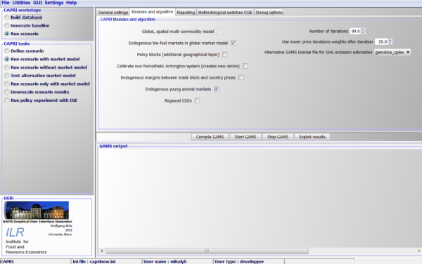
The Witzke et al. approach is implemented in a modular fashion in the CAPRI market model. The calibration of the modified Armington lower nest can be switched on or off through a designated button on the CAPRI GUI (see the next Figure). In order not to interfere with the work of other CAPRI users, a specific GUI is created for the project that can be started by running GUI\capri64modarm.bat.
Figure 21: GUI Option for the non-homothetic Armington system
The calibration of the non-homothetic Armington demand system does not require a full re-calibration of the complete CAPRI modelling system; it can be found under the workstep “Run scenario”, task: “Run scenario with market model”. Technically, the calibration modifies the simini\sim_ini.gdx file that contains the necessary starting parameters for a CAPRI simulation: if the above GUI option is selected then the existing sim_ini.gdx file is automatically deleted and the create_sim_ini CAPRI module is called. This is all steered in the main capmod.gms file by a specific GAMS setglobal variable called modArmington:
The calibration model itself is called directly by the arm\market1.gms file:
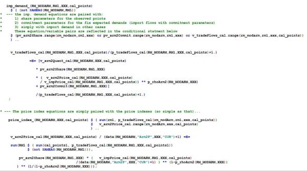
The file arm\modArmington.gms file contains the definition of the calibration model and executes the calibration itself. The calibration model simply consists of Armington share equations (importShares_) and price index equations (arm2PriceAgg _), following the approach presented above.
The share- and price index equations of the calibration model are similar to those in the CAPRI market model, but extended with an additional dimension called ‘cal_points’. The additional dimension indicates whether the equations correspond to the observed or the expected calibration points. The arm\modArmington.gms file calculates the expected price/quantity framework necessary for the Witzke et al. approach. The data input for this calculation is currently implemented in the scenario file in order to allow for a compact definition of baseline and scenario assumptions. The test scenario for the Witzke et al. demand system assumes the following expected EU poultry imports from the US under a hypothetical import price:
The calibrated share equations and the commitment terms are then stored in the appropriate parameters and later picked up by the market model. The relevant equations of the market model, therefore, also had to be modified. For example, the Armington share equations of the CAPRI market model are extended with the commitment term (p_arm2Commit = \(\mu\)):
The calibration of the full market model is tested by solving the model at trend values in the CAPRI module arm\prep_market.gms. This module also had to be modified in order to initialize the modified Armington system appropriately. The modifications mostly affect the trade flows, import prices and trade policy instruments.
If properly calibrated, the modified Armington system with the test reference scenario should replicate the standard baseline results. It means, for example, that emerging trade flows being zero in the baseline will remain zero in the reference run and only become positive under specific scenario assumptions.
Biofuel module
An achievement of the CAPRI biofuel module is that biofuel supply and feedstock demand react flexibly to the price ratio of biofuel and feedstock prices as well as biofuel demand and bilateral trade flows react flexibly to biofuel prices and further relevant drivers.
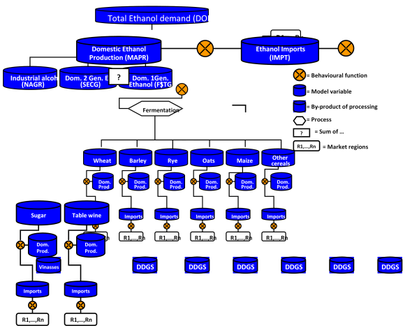
Figure 22: Construction of the ethanol market implemented in CAPRI 
Soruce: Capri Modelling System
Basically two biofuel product markets are covered in the model; Ethanol (BIOE) and Biodiesel (BIOD). For total domestic ethanol production, three technology pathways are covered; 1st generation ethanol (BIOFE) - differentiated in wheat, barley, rye, oats, maize, other cereals, sugar and table wine, 2nd generation ethanol (SECG), and non-agricultural ethanol (NAGR).
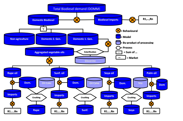
A similar technological pathway for biodiesel production has been implemented as shown in Figure 22. The three production pathways for biodiesel are; 1st generation biodiesel (BIOFD) produced from vegetable oils (rape oil, sunflower oil, soya oil, and palm oil), 2nd generation biodiesel (SECG); and non-agricultural biodiesel (NAGR).
Figure 23: Construction of the biodiesel market implemented in CAPRI
Soruce: Capri Modelling System
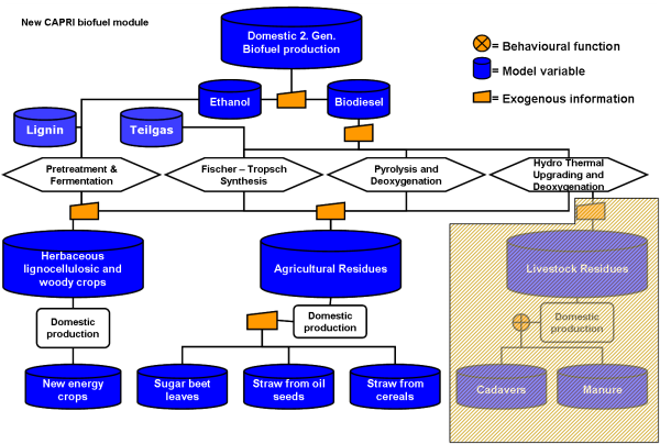
The figure below provides a schematic diagram of the process of 2nd generation biofuel production in CAPRI. Two different product aggregates are introduced in the CAPRI product list to cover feedstock for 2nd generation biofuel processing:
- A product aggregate for agricultural residues (ARES) which covers straw from cereals and oil seed production and sugar beet leaves and
- A product aggregate for new energy crops (NECR) which cover herbaceous and woody crops like poplar, willow and miscanthus.
The use of residues from livestock production, which covers manure and cadavers, is not included in the second generation processing as this source is assumed to have only a marginal importance for biofuel processing, Furthermore, the demand shares for the single agricultural residues are provided exogenously in the model. This assumption relies on the observation that the potential of ARES resulting from the activity levels of cereals, oilseeds and sugar beet production in the base and projection year is so high that even in a high second generation scenario (50% of biofuel demand in EU should be stemming from 2nd generation biofuel processing) could only generate a demand of up to max. 10% of the actual potential. The demand share for new energy crops in the second generation production quantities is also provided exogenously in the model. However, as the production of new energy crops require agricultural land the available agricultural land for the production of other agricultural products is reduced accordingly with the yield information collected for NECR.
Figure 24: Consideration of 2nd generation biofuel production and related feedstock
Biofuel supply and feedstock demand
Biofuel feedstock demand is driven by per unit net input costs (µ). These are defined per ton of input used and are calculated for each feedstock in a country by feedstock price minus by product revenues per ton of input.
\begin{equation} \mu_{r,xf} = p_{r,xf}- \sum_{xbp} p_{r,xbp}\alpha_{r,xf,xbp} \end{equation}
The index r contains all regions in the market module that have biofuel production. All feedstocks that can be used to produce first generation biofuels are stored in the index xf and the by products Glycerine, DDGs and Vinasses in xbp. Prices are denoted by p. One speciality exists in the case of sugar prices in the EU, where a specific ethanol sugar price is assumed in case of the existence of production quotas. This is due to the fact that ethanol beet in the EU purchased at a lower price than beets processed to sugar. These single feedstock costs then form a CES aggregate to give the average cost for the respective biofuel:
The index r contains all regions in the market module that have biofuel production. All feedstocks that can be used to produce first generation biofuels are stored in the index xf and the by products Glycerine, DDGs and Vinasses in xbp. Prices are denoted by p. One speciality exists in the case of sugar prices in the EU, where a specific ethanol sugar price is assumed in case of the existence of production quotas. This is due to the fact that ethanol beet in the EU purchased at a lower price than beets processed to sugar. These single feedstock costs then form a CES aggregate to give the average cost for the respective biofuel:

The superscript c indicates the average input costs in the calibration point which are only introduced to have price variables “around one” in the expression to help the solver.
The decision on the total biofuel production happens simultaneously with the decision on the optimal feedstock mix. The latter is based on the FOC of cost minimisation with a CES cost function for a given biofuel output:
\begin{align} \begin{split} fd_{r,xf} &= \phi_{r,xf}x_{r,xb}^{1st} \left [ \frac{\mu_{r,xb}}{\mu_{r,xf}}\right]^{\rho_{r,xb}} \quad \forall xf\ne num \\ s.t. \quad &\rho_{r,xb} =\frac{1}{(1-\sigma_{r,xb})}-1 \end{split} \end{align}
The subsitution elasticity of the CES function is given by σ and their share parameters by \(\phi\). First generation biofuel procuction (\(x^{1st}\)) is then derived by the product sum of feedstock demand fd and their biofuel processing coefficinents:
\begin{equation} x_{r,xb}^{1st} = \sum_{xf} fd_{r,xf} \alpha_{r,xf,xb} \end{equation}
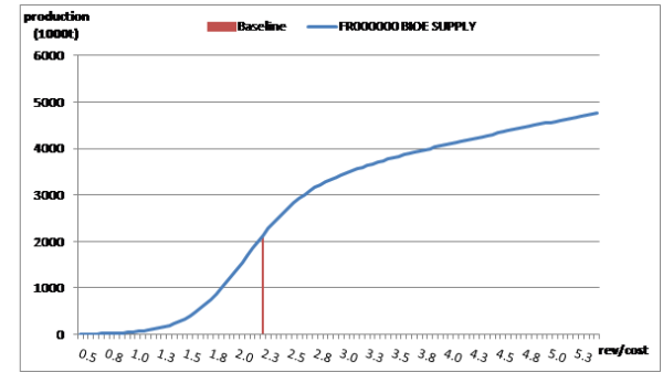
For biofuel supply from first generation technologies (\(x^{1st}\)) a function of the relation of the respective biofuel price and the corresponding average feedstock per unit costs has been specified. A synthetic supply function was chosen that satisfied some plausibility considerations, which were 1) that supply strongly decreases when the the price relation gets below a certain “trigger” value and that this strong slope is not maintined throughout the whole function.
\begin{align} \begin{split} x_{r,xb}^{1st} = \begin{bmatrix} \partial_{r,xb}\frac{p_{r,xb}}{\mu_{r,xb}} \\ +exp \left ( \beta_{r,xb}^{1} +\beta_{r,xb}^{2} ln\left ( \frac{p_{r,xb}}{\mu_{r,xb}}\right)\right)\frac{1}{1+exp\left (\left (\frac{p_{r,xb}}{\mu_{r,xb}}-\delta_{r,xb}^{1}\right)\delta_{r,xb}^{2}\right)} \end{bmatrix} \end{split} \end{align}
This function consists of three parts on the RHS: the first part is linear (a small positive value for δ), the second part is semi-log and the third is sigmoid. The linear term guarantees a minimal slope, where the sigmoid function would return a slope of almost 0. The semi-log term is active at processing margins considerably higher than in the baseline point and the sigmoid function guarantees a steeper slope in a range where processing starts and production is close to zero when feedstock costs exceed output values. The coefficients β and δ are behavioural parameters in these functions. All biofuel supply equations are generally of the style presented below with an example of bioethanol in France.
Figure 25: Biofuel supply function in France
The supply of by products is directly linked to the first generation biofuel output:
\begin{equation} x_{r,xbp} = fd_{r,xf} \alpha_{r,xf,sbp} \end{equation}
Total biofuel output is then defined as the sum over first generation, second generation (secg), non agricultural (nagr) and some exogenous production (exo) from products not mapped to the feedstocks in CAPRI (only relevant in extra EU countries):
\begin{equation} x_{r,xb}^{tot} = x_{r,xb}^{1st} +x_{r,xb}^{secg}+x_{r,xb}^{nagr}+x_{r,xb}^{exo} \end{equation}
Biofuel demand
The representation of biofuel demand was simplified compared to the approach chosen first and applied in Becker (2011). There the Aglink demand system was more or less reproduced using a different functional form but keeping the three types of biofuel demand, the use as additive, as low blends and in flexible fuel vehicles. The actual biofuel demand equations consist of only one sigmoid function instead of stacking three of them. The share of biofuel in total fuel demand (bsh) is hereby defined as:
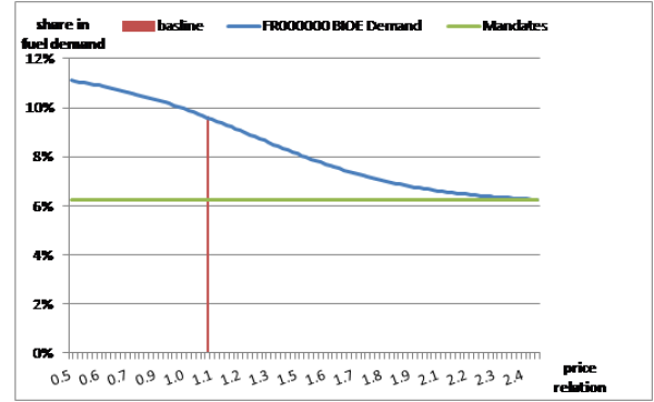
\begin{equation} bsh_{r,xb} = bsh_{r,xb}^{q} + \frac {bsh_{r,xb}^{max}}{1+exp\left (\left (\frac{p_{r,xb}}{p_{r,f}}-X_{r,xb}^{1}\right)X_{r,xb}^{2}\right)} \end{equation}
Again the coefficients X are used to specify the exact slope of these functions. The first term (bshq) defines the part of the biofuel demand which is enforced by any kind of obligation quota or mandate, while the second part defines an “endogenous” part of the demand. This term has the upper linmit \(bsh_{max}\) which represents the maximum biofuel share on top of the quota obligation that is deemed reachable in a certain country. The endogenous demand component is driven by the price relation of a biofuel ( \(p_{r,xb}\)) to the respective fossil fuel substitute ( \(p_{r,f}\)). These demand share functions are of the type represented by the example of France below:
Figure 25: Biofuel demand share function in France
Total biofuel demand (\(d_{r,xb}\)) is then derived by multiplying this share to the exogenous total fuel demand (\(d_{r,f}\)):
\begin{equation} d_{r,xb} = bsh_{r,xb} +d_{r,f} \end{equation}
Total fuel demand
Total fuel demand is exogenous to the CAPRI model. However, an econometric estimation was undertaken to receive a demand reaction on exogenous drivers like the oil price and GDP. This function can then be used in Scenarios to adjust total fuel demand, if these drivers are altered. A response surface estimation on the basis of available PRIMES scenarios from 2008 was undertaken. The PRIMES output files at hand allow for estimating the relation between total fuel demand, GDP and fossil fuel prices. For the estimation an ordinary least square estimator is used. A double log demand function is chosen where the estimation coefficients can directly be interpreted as elasticities. The regression function and thereby the total fuel demand function is defined by:
\begin{align} \begin{split} log(y_{i,j,s,t}) = \delta_{i,j} &+ \alpha_{i,j} \, log(p_{i,j,s,t}) + \beta_{i,j} \, log(gdp_{j,s,t}) \\ &+\gamma \, log(trent_{t}) + \epsilon_{i,j,s,t} \end{split} \end{align}
where,
i = Fuel type
r = Region
s = Scenario
t = Year
y = Fuel demand
p = Fuelprice including tax
gdp = Gross Domestic Product
trend = Trend variable
\(\epsilon\) = Error term for regression
\(\delta\) = Intercept
\(\alpha\) = price elasticity of demand
\(\beta\) = GDP elasicity of demand
\(\gamma\) = Trend elasicity of demand
The results of the regression analysis (differentiated into biodiesel and ethanol for every EU MS) cover estimates for α, β, γ and the intercept (δ). The significant estimates are used directly in the respective fuel demand function. If no significance was observed for a coefficient in a respective country, the estimated value is replaced by an average value which is derived from the weighted average of significant coefficients over all EU MS. The resulting matrix of regression coefficients (elasticities) in the fossil fuel demand function are displayed in table below. As the PRIMES data only covers values for European countries but also estimates for the non-European CAPRI regions are required it was assumed that the coefficient estimates for the aggregated EU27 are also applicable for those regions.
Assumed elasticities for total fuel demand after filling with average values are demonstrated in the table below.
Table 29: Overview of pillar II measures modelled in CAPRI 

Source: Own calculation based on PRIMES 2009
Biofuel Trade
Behavioural functions for global bilateral trade of biodiesel and ethanol are intrinsically tied to the final biofuel demand functions. The general methodology is that of a two stage demand system relying on the Armington assumption as already applied for other agricultural commodities in the standard CAPRI version. Biofuel demand for fuel use is considered a derived demand of refineries and responsive to the price ratio of biofuels to fossil fuels. The non fuel demand for biofuels (e.g. ethanol demand of the chemical industry) is consequently set on INDM or PROC (industrial use).
Calibration of the biofuel system
So far, only the general form of the biofuel supply and demand functions where derived, but without any adjustments, they won’t reproduce the biofuel price-quantity framework of our baseline. Therefore both behavioural functions are due to a calibration process which takes place in ‘gams\biofuel\def_biofuel_params.gms’.
Firstly, the demand system is calibrated. We here assume that only the part of the observed biofuel demand share in total fuel demand that is above the quota obligations is the result of a consumer decision and thus a result of the flexible parts on the demand equations. To calibrate the demand functions to the observed combination of the price ratio bio- to fossil fuel and demand share in total fuel consumption, we chose the two parameters \(X^1\) and \(X^2\) such that:
- It recovers the baseline combination of price and quantity relations
- It reaches 90% of the max share (\(bsh_{max}\)) at a certain price relation (currently 0.5 for ethanol and 0.3 for biodiesel)5).
The maximum biofuel demand share of a region is chosen 2% above the observed baseline share.
The parameters \(\beta^2\), representing the supply elasticities of the double log part of the biofuel supply equation were chosen at 0.56). For the two δ parameters the following rules were applied: δ1, representing the turning point of the sigmoid function was defined to be left to the calibration point at 90% of the processing margin of the baseline. The slope parameter \(\delta^2\) defines in which range the sigmoid function increases from 0 to 1. A higher value corresponds then to a steeper slope. Assuming that countries with higher processing margin are more competitive, we assume a higher slope for lower processing margins. Furthermore in non-EU countries we assume the functions less steep. Finally the parameter \(\beta^1\) is chosen such that the baseline is reproduced.
Endogenous policy instruments in the market model
Subsidised exports
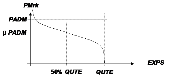
On the market side, the amount of subsidised exports (exps) are modelled by a sigmoid function, driven by the difference between EU market (pmrk) and administrative price (padm), see equation below. The sigmoid function used looks like:
\begin{equation} Sigmoid(x)= exp \frac {min(x,0)}{1+exp(-abs(x))} \end{equation}
where x is replaced by the expression shown below in the equations.
The response was chosen as steep as technically possible by setting a high value for \(\alpha\), i.e. intervention prices are undercut solely if WTO commitment (QUTE) and the maximum quantity of stock changes are reached.
\begin{equation} expsVal_{i,r} = QutE_{i,r} \left [sigmoid \left( \frac {\alpha_{i,r}}{PADM_{i,r}}(v\_marketPrices_{i,r}-\beta_{i,r}^E PADM_i)\right ) \right] \end{equation}
The parameters \(\alpha\), \(\beta\) are determined based on observed price and quantities of subsidised exports. The per unit subsidy is defined from non-preferential exports and the value of the subsidies:
\begin{equation} expSub_{i,r} = 1000 expsVal_{i,r}/ v\_nonDoubleZeroExports_{i,r} \end{equation}
The relation is shown in the figure below.
Figure 27: Modelling of subsidised export costs by a logistic function
Endogenous administrative stocks
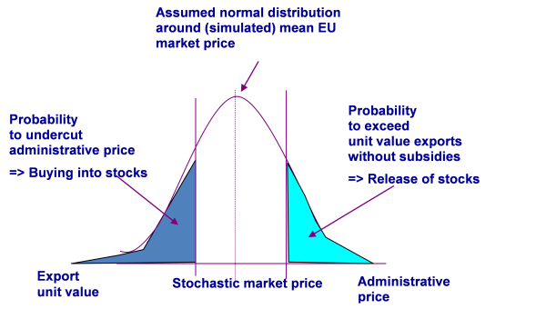
For years, the CAP defended administrative prices in key markets such as cereals, beef, butter and skim milk poweder by direct interventions into markets which where out into public stocks. The basic functioning of that mechanism in CAPRI in shown in the figure below.
Figure 28: Endogenous administrative stocks in CAPRI
Purchases to intervention stocks v_buyingToIntervStock depend on the probability of the current market price v_marketPrice to undercut the administrative price padm and a calibration parameter \(\gamma^p\), assuming a normally distributed market price with standard deviation stddev and maximal amounts of purchases INTM:
\begin{equation} v\_buyingToIntervStocks_{i,r} = INTM_{i,r} errf\left ( \left( padm_{i,r} - v\_marketPrice_{i,r} + \gamma_{i,r}^p\right ) / stddev_{i,r} \right ) \end{equation}
A decrease of the administrative price or an increase of the market price will hence decrease purchases to intervention stocks.
Releases from intervention stocks v_releaseFromIntervStock depend on the probability of market prices v_marketPrice to undercut unit value exports uvae and a calibration parameter , \(\gamma^p\), multiplied with the current intervention stock size being equal to starting size intk plus intervention purchases intp:
\begin{equation} intd_{i,r} = (intk_{i,r}+intp__{i,r}) errf \left ( \left( uvae_{i,r} - pmrk_{i,r} + \gamma_{i,r}^p\right ) / stddev_{i,r} \right ) \end{equation}
Releases will hence increase if world market price increases or the EU market price drops, and if the size of the intervention stock increases. The parameters \(\gamma\) are determined from ex-post data on prices and intervention stock levels. The change in intervention stocks ints entering the market balance is hence the difference between intervention purchases intp and intervention stock releases intd:
\begin{equation} ints_{i,r} = intp_{i,r} - intd_{i,r} \end{equation}
Endogenous tariffs under Tariff Rate Quotas, flexible levies and the minimum import price regime for fruits and vegetables of the EU
Tariff Rate Quotas
Tariff Rate Quotas (TRQs) establish a two-tier tariff regime: as long as import quantities do not exceed the import quota, the low in-quota tariff is applied. Quantities above the quota are charged with the higher Most-Favoured-Nation (MFN) tariff. CAPRI distinguishes two types of TRQs: such open to all trading partners, and bi-laterally allocated TRQs. As a rule, bi-lateral allocated quotas are filled first. Equally, as for all tariffs, TRQs may define ad valorem and/or specific tariffs.
A market under a TRQ mechanism may be in one of the following regimes:
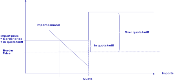
Quota underfill: the in-quota tariff is applied. The willingness to pay of the consumers is equal to the border price plus the in-quota tariff.
Figure 29: Quota underfill regime
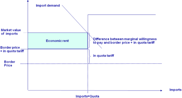
Quota binding, i.e. exactly filled: the in-quota tariff is applied. The willingness to pay of consumers and thus the price paid is somewhere between the border plus the in-quota tariff and the border price plus the MFN tariff. The difference between the price in the market and the border price plus the in-quota tariff establishes a quota rent. Depending on property rights on the quota and the allocation mechanism, the quota rent is shared in different portions by the producers, importing agencies, the domestic marketing chain or the administration. Typically, the quota rent can neither be observed nor is their knowledge about distribution of the rent.
Figure 30: Quota binding regime
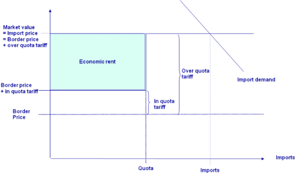
Quota overfill: the higher MFN-tariff is applied. The quota rent is equal to the difference between the MFN and the in-quota tariff. Again, how the quota rent is distributed to agents is typically not known.
Figure 31: Quota overfill regime
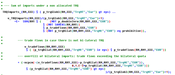
The fill rate for global TRQs is defined in the code as follows, adding all imports which are not under no duty/not quota access (p_doubleZero), not from the same trade block and not prohibited. A special case provides a bi-lateral quota, here, only import quantities beyond the allocated quota quantity enter the global one.
There are a couple of further complications, linked to spatial and commodity aggregation problems. In many cases, TRQs are defined for very specific data qualities, which are more dis-aggregated as the product definition of the model. TRQs for beef may refer e.g. to specific cuts, races or even feeding practises. That typically leads to a situation where both imports covered and not covered by a TRQ mechanism are aggregated in the data base of the model. Consequently, it is not clear, which regime governs the market. Further on, TRQs may be defined for individual countries where the model works on a country block.
Besides the problem of defining the regime ex-post, the relation between the import quantity and the tariff is not differentiable but kinked. Therefore, again a sigmoid function is applied in the CAPRI market part:
In many cases, the EU features for the very same market so-called bi-lateral quotas and market access quotas from the URA round which must be open to all imports (“erga omnes”). As the allocation shares for the latter are currently not know to the CAPRI team, any importer is allowed to import under these global TRQs. Importers have bi-lateral quotas might import under global TRQs once the bi-lateral TRQs are overshot.
Flexible tariffs
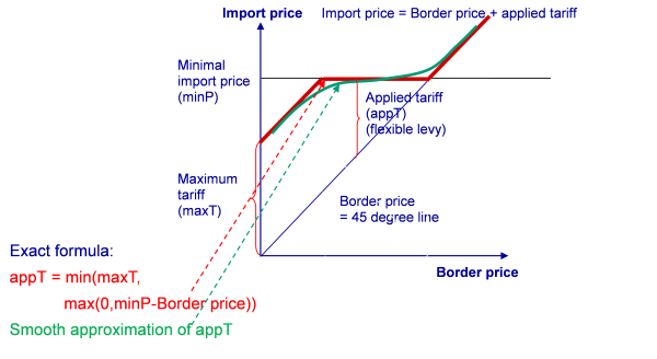
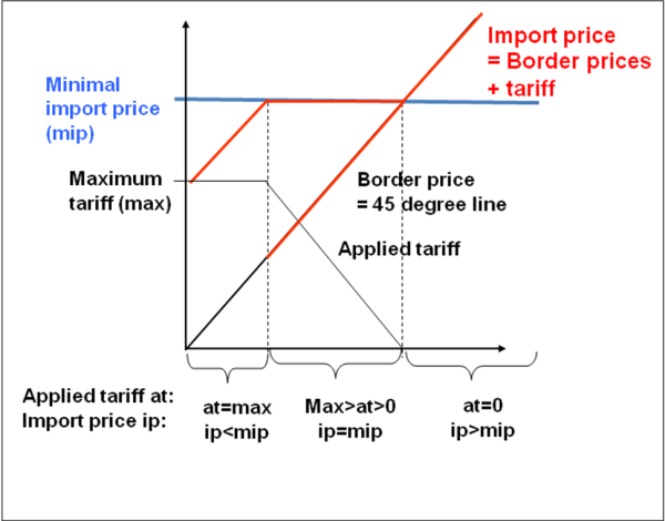
Geneally, the WTO rules only set upper bounds on the tariffs (so-called Most Favorite Nature or MFN for short rates), but allows its members to reduce the tariffs as long as the same tariff is applied for all WTO members. Exemption from MFN rates which are implemented in CAPRI are preferential rates for Developing countries (Everything But Arms agreement of the EU), Free Trade Agreements and bi-lateral concessions e.g. results from minium market access obligation from the Uruguay rounds under TRQ. The EU generally uses MFN rates, but operates in the cereal markets a specific form of a variable tariff called the “levy” system. The last WTO EU trade policy review described the operation of the CAP import regime for cereals as follows: “In response to fluctuations in world prices, the EU has, within the limits of its bound tariffs, changed its MFN applied tariffs. It reduced tariffs on cereals to zero in January 2008 in response to high world prices, and reintroduced them at the end of October 2008. For wheat, the tariff is based on the difference between world prices and 155% of the intervention price, up to the bound rate of €95 per tonne for high quality wheat and €148 per tonne for high quality durum wheat with similar systems for other cereals.”
Figure 32: Variable levies
In CAPRI, the system is implemented as follows:
\begin{equation} v\_flexLevy_{i,r} = min \left [ v\_tarSpec_{i,r} , max(0,minBordP_{i,r}-cif_{i,r})\right ] \end{equation}
The actual implementation in the code differs somewhat, as the min and max operators are replaced by “fudging function”, and the cif price is expressed as a term from several variables and constants instead of being a separate variable. The first expression is equivalent to the max(0,minBord-cif) expression above:
The second equation defines the actual tariff applied:
Entry price system for fruits and vegetables
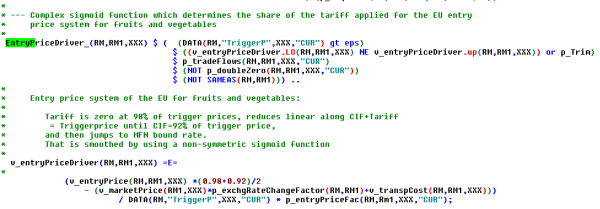
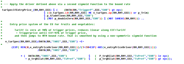
A somewhat similar instrument is the entry price system used in the fruit and vegetable sectors of the EU. The entry price relates the applied tariff to a specified trigger price in a way that encourages imports at a price (CIF plus tariffs) that is between 92% and 98% of the trigger price.
Figure 33: EU entry price system for fruits and vegetables
In order to implement the system, first the difference beween 96% of the entry price and the cif in relation to the triggerprice is defined, times a possible factor to ease solution.
That factor is the fed into a modified sigmoid function which as a result approximates the relations in the graphic shown above:
Tariff computation in the model
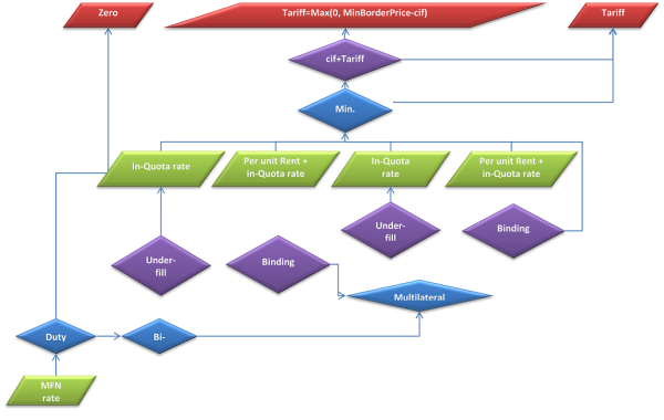
The figure below depicts the interaction of the various elements of the tariff calculation discussed above. The blue boxes are policy instruments depicted in the model; the purple ones describe endogenous switches and the green ones intermediate model variables which can be interpreted as intermediate results for the applied tariffs. The red boxes show the rate applied to derive the import price. Arrows upwards from a decision box mean yes, to the left no.
The simplest decision is in the left lower corner: a check if the importer benefits from duty and quota free accesss. Examples are intro-EU trade or import from LDCs into the EU under the “Everything But Arms”-Agreement. If that is the case, the applied tariff is zero.
Next we check for a bi-lateral TRQ. If we find one, we check if it is underfilled in which case we apply the in-quota rate. Next we check if the quota is just binding, in which case the applied rate represents the sum of the in-quota rate and an endogenous per unit quota rent. The remaining case is that of a quota overfill where we are left with the MFN rate.
Next we check for a multi-lateral TRQ, also in case we have an overfilled bi-lateral TRQ. If we find one, we check if it is underfilled in which case we apply the in-quota rate. Next we check if the quota is just binding, in which case the applied rate represents the sum of the in-quota rate and an endogenous per unit quota rent. The remaining case is that of a quota overfill in which case the MFN rate is applied.
In all cases for specific tariffs, the results applied rates are checked against the existence of a minimum border price system. In that case, the import price resulting from applying the tariff to the cif price is compared to the minimum price. If it is higher than the minimum price, the tariff is cut such that the import price becomes equal to the minimum border price as long as the resulting tariff does not become negative.
Figure 34: Tariff computation in the model
Welfare-consistent tariff aggregation module
The heterogeneity of trade policies across different traded goods generates a serious index number problem for large-scale applied equilibrium modelling. Trade policies must be described with aggregate indices in order to incorporate them in the aggregate commodity structure of applied equilibrium models. Even though the CAPRI commodity coverage is quite detailed in comparison to other applied equilibrium models of global agri-food trade, tariff policies are usually defined and applied at an even finer level of details, i.e. at the tariff line level. In order to improve on the state-of-the-art in CAPRI, an advanced tariff aggregation module has been developed recently in a JRC-IPTS study (154208.X1) than may be switched on demand (and it the required data are avilable). The stand-alone tariff aggregation module aggregates tariffs and Tariff Rate Quotas (TRQ) defined at the HS tariff-lines into an ad valorem equivalent tariff rate at the level of commodities in the CAPRI market module.
Review of current tariff aggregation approach in CAPRI
The tariff aggregation in CAPRI is based on the weighted average method, but applies a combination of different weights in order to (1) overcome the endogeneity bias and to (2) correct for outliers that are frequently created by statistical errors in the trade data. Technically, the tariff aggregation is performed in the module responsible for creating the global database for the market model. The main information source is the AMAD7) database providing applied and bound tariffs as well as import statistics of agricultural commodities at the HS6 level. Unfortunately, the AMAD database does not contain bilateral trade statistics. Therefore additional trade statistics had to be requested and added to the CAPRI system (see below).
Although Tariff Rate Quotas (TRQ) are typically defined in the legal texts over tariff lines, the CAPRI database does not contain data on TRQs at that level of product aggregation. In fact, TRQs are defined in CAPRI at a much more aggregated commodity level. As a consequence, tariffs under TRQ must be aggregated on an ad-hoc basis to the CAPRI commodity nomenclature before they enter the system. The advanced tariff aggregation module provides an alternative by calculating aggregate tariff equivalents of TRQs systematically, taking into account a more detailed tariff and TRQ structure at the HS6 level.
Advanced tariff aggregation techniques considered
The two fundamental obstacles to aggregate tariffs and other border protection measures are
- The conversion problem, i.e. different policy instruments need to be expressed in a common metric before they can be aggregated
- The index number problem, i.e. individual trade restrictions must be appropriately aggregated (weighted)
A large number of tariff aggregation techniques are available in the literature, each having its specific objective, drawbacks and merits. Cipollina and Salvatici 2008 provide a typology for the aggregate measures of border protection:
- Incidence measures are based on the intensities of the policy measures, and are derived only from direct observations on policies. They do not consider the distortive effects of the trade policies on the economy. Typical incidence measures are tariff dispersion or the frequency of various types of Non-Tariff Measures.
- Outcome measures incorporate other variables than policy variables in order to take into account the distortive impacts of policies on the economy. Typical outcome measures include trade weighted average tariffs. Outcome measures remain 'a-theoretic' in a sense that they do not meet any equivalence criteria.
- Equivalence measures provide aggregates that are equivalent to the original data in terms of selected economic variables. Welfare-consistent measures, for example, provide aggregates that are equivalent in their impact on selected indicators of the the economy's welfare (e.g. real income). In order to derive equivalence measures, explicit model structures (supply/demand structures) must be assumed and parameterized.
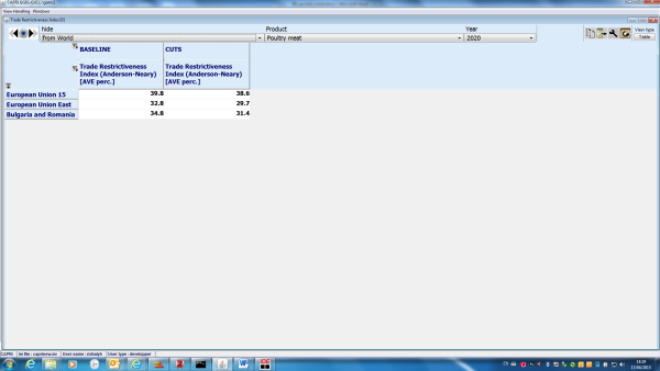
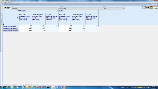
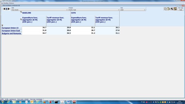
The advanced tariff aggregation module provides three welfare-consistent aggregators: Bach-Martin approach, Anderson's optimal tariff combination and the Trade Restrictiveness Index (TRI). The procedure developed by Anderson (2009) combines two indicies in a modified balance-of-trade condition for welfare-consistent tariff aggregation. The trade weighted average tariff is combined with the 'true average tariff'. The true average tariff is the tariff aggregator that consistently generates total aggregate trade volume and aggregate prices. The true average tariff alone does not allow for welfare consistent aggregation in the general equilibrium framework. It needs to be combined with the trade weighted average tariff in order to calculate tariff revenues and hence real income correctly. This inconsistency issue has been first raised and addressed by Bach and Martin (2001). They used a revenue constant uniform tariff together with a trade-expenditure constant uniform tariff, as the basis of a compensating variation approach for tariff aggregation. Their approach, however, is only consistent in the one-country case. In the multi-country setup their welfare-analysis fails, because global payments do not balance. One of the key contributions of Anderson (2009) is exactly the solution he provides for the global balance problem. The TRI of Anderson and Neary (1994) preserves real income in shifting from the tariff line structure of trade policies to a single uniform ad-valorem tariff. The TRI is a commonly used measure of aggregate protection, specifically useful for comparing protection level across countries. The implementation of the welfare-consistent tariff aggregators closely follow Himics and Britz, 2014 which includes an extension of the original methods to the case of TRQs. As a result, the tariff aggregation module is able to handle ad-valorem and specific tariffs as well as TRQs at the tariff line level.
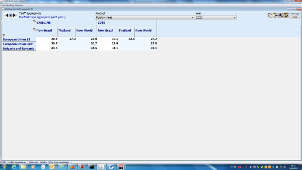
A traditional outcome measure, called the MacMap-type aggregator, is also available in the tariff aggregation module. The aggregator is named after the conversion rule for TRQs, which is the same as the one underlying the MacMap database: TRQs are converted to an ad-valorem equivalent based on the fill rate of the TRQ. This approach takes into account the quota rent generated by the TRQ, but defines its level arbitrarily (the unit quota rent is set to half of the difference between out-of-quota and in-quota rates).
Additional data requirement and its integration in CAPRI
An extraction from the UN-COMTRADE database has been integrated in the global module of CAPRI. The dataset comprises of import values and calculated unit prices for 326 tariff lines (mainly agricultural commodities), covering 79 reporting and 99 partner countries, for the years 2007-2013.
A major difficulty arises when we use raw UN-COMTRADE data for modelling purposes, due to their lack of symmetry. Country A’s import of a given product from country B is not the same as country B’s export of that product to country A. The literature identifies three main causes for this discrepancy (McCleery and DePaolis, 2014):
- An obvious wedge between import and export values is created by the valuation of exports at point of origin (usually f.o.b. prices) and the valuation of imports at destination (mostly c.i.f. prices).
- Border disputes, export bans or prohibitive trade restrictions may lead to only one half of the trade transactions being recorded.
- Border frictions may also lead to distorted trade statistics, e.g. large discrepancies in the US-China trade statistics can be observed due to recording trade with Hong-Kong differently
This problem is currently solved by using UN-COMTRADE data only on imports, applying the assumption that countries tax and regulate imports more thoroughly than exports.
The only source of trade policy data at the tariff line level in the current CAPRI system is the AMAD database. AMAD is not anymore updated by OECD, and in many respect contains outdated policy information. According to the Technical Specification, the current study relies on the AMAD data, and does not include and update of trade policies at the tariff line level. This is a clear limitation that should be improved on in the future. It is very likely that a combination of additional trade policy databases need to be added to CAPRI for a correct and comprehensive representation of global trade policies at the tariff line level. MAcMap is one of the candidates to be included, containing global trade protection measures at HS6 level. MAcMap, however, contains TRQs already in a converted tariff-equivalent form, and is therefore insufficient to provide policy data for the explicit TRQ mechanism in the new tariff aggregation module.
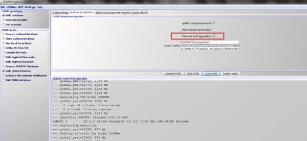
The code implementation of the UN-COMTRADE data processing is modular, i.e. it can be switched on and off upon demand. A dedicated option in the GUI activates the data processing algorithms in the global part of CAPRI (see below). Technically, the extended GAMS routines create an additional intermediate dataset (‘\global\tariff_aggregation.gdx’) that is a direct input of the tariff aggregation module in subsequent steps. The .gdx file contains bilateral trade and tariff information at the tariff line level, already mapped into the CAPRI regional nomenclature.
Figure 35: Tariff computation in the model
Source: CAPRI Modelling System
The different tasks implemented in the aggreg_tariffs.gms tariff aggregation module includes:
- Defining nomenclatures and sets for the UN-COMTRADE dataset (‘global\comtrade_sets.gms’)
- Processing, filtering and mapping UN-COMTRADE data in order to align it with the CAPRI database
- Aggregate tariffs to the CAPRI regional nomenclature. The aggregation follows the standard CAPRI approach; the only difference is that tariffs are not aggregated over tariff lines.
Unit values in the UN-COMTRADE dataset have been found to be subject to significant statistical errors. An outlier-detection algorithm has been therefore implemented in order to tackle this problem. Using a simple and robust approach, observations outside a given range around the mean are identified as outliers and replaced with the mean. The outlier detection is implemented in R8), and can be easily combined with other outlier detection algorithms. Improvements of outlier detection algorithms (subject to future research) can further increase the accuracy of the tariff aggregation. Technically, the GAMS code automatically communicates with the outlier detection algorithms in R, and performs the data checks on the raw UN-COMTRADE data.
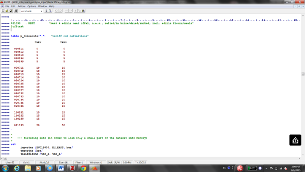
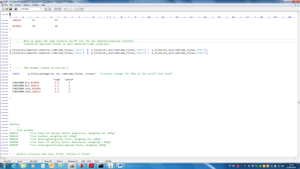
Defining Tariff cut scenarios at the tariff line level
The tariff aggregation module is loosely linked to the CAPRI modelling system. The feature can be activated by a GUI option (see below), assuming that the intermediate database has been already created by the global module.
Figure 36: Activation of the tariff aggregation module on the GUI
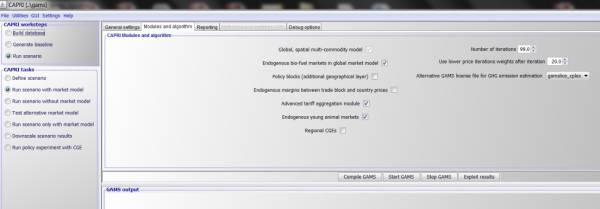
Source: CAPRI Modelling System
The tariff aggregation module takes over the appropriate tariff cuts from the scenario file and applies them at the tariff line level. The module then feeds back an aggregate tariff equivalent of the resulting (cut) tariffs.
CES demand structure
With specific assumptions on the demand side, it is possible to take into account the changes in the consumption bundle, as a response to relative price changes induced by the tariff cut scenario. Loosely speaking, the tariff aggregation module takes into account the substitution between goods within an aggregated CAPRI commodity, under specific assumptions on the demand structure. We assume a nested CES import demand structure on the lines of the usual Armington approach to model bilateral imports with cross-hauling. The current implementation is a “small country” approach: tariffs are aggregated for one importer region after the other, assuming fix border (c.i.f.) prices.
Dropping the small country assumption would require a full partial equilibrium model at the tariff line level for the commodity considered, as done in e.g. Grant et al. (2007). This, however, requires a substantial extension of the CAPRI database by including tariff line-specific trade and trade policy information at the global scale. The complexity of the market model would increase rapidly by adding trade flows at the tariff line level. A simultaneous solve for all commodity markets would be technically impossible. No surprise that similar examples in the literature only focus on selected markets and do not implement a full-fledged market model with many interacting markets at the tariff line level. Grant et al. (2007) focus on the dairy market only, and implements a sequential model linkage in order to reduce the computational requirements of solving the complete system whereas Narayanan et al. (2010) extend the standard GTAP model with a partial equilibrium component that only covers the automobile industry.
Technical details of implementing tariff aggregation scenarios
Generally, tariff cuts have to be defined in a specific format in the CAPRI scenario file. A simple example is illustrated in hte following, where ad-valorem and specific tariffs are cut relative to their initial level and TRQ thresholds are increased.
Reporting (GUI tables)
The GUI has been extended with tables under 'Trade|Advanced tariff aggregators' that collect the results of the tariff aggregation module:
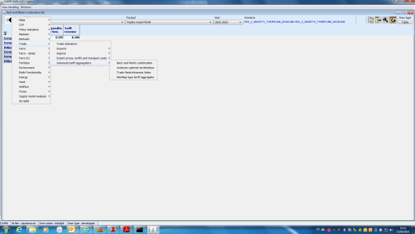
Source: CAPRI Modelling System
The MacMap-type aggregators are calculated both with respect to bilateral trade relations and with respect to a total ('from World') measure of tariff/TRQ restrictions. In the above calculation of total aggregate measures, imports from other countries are neglected; an assumption that can be easily relaxed if relevant policy and trade data will be available in future applications. MacMap-type trade weighted aggregators give the following results.
TRI estimates are also reported in a specific GUI table. By definition the TRI indicies are defined for all trade relations only (not a bilateral index):
The Anderson tariff combination is presented next. The current implementation is an extension of the original approach, including correction factors for TRQs (Himics and Britz, 2014):
The Bach and Martin (2001) approach, i.e. a combination of an aggregator for the expenditures and another one for the tariff revenues, is also implemented and reported in a designated GUI table:
Overview on a regional module inside the market model
The resulting layout of a market for a country (aggregate) in the market module is shown in the following diagram. Due to the Armington assumption, product markets for different regions are linked by import flows and import prices if observed in the base year. Accordingly, no uniform world market price is found in the system.
Figure 37: Graphical presentation for one region of a spatial market system
Basic interaction inside the market module during simulations
As with the supply module, the main difficulty in understanding model reactions is based on the simultaneity of changes occurring after a shock to the model. Cross-price effects and trade relations interlink basically all product markets for all regions. Whereas in the supply model, interactions between products are mostly based on explicit representation of technology (land balances, feed restrictions), such interactions are captured in multi-commodity models in the parameters of the behavioural functions.
Even if the following narrative is simplifying and describing reactions as if they would appear in a kind of natural sequence where they are appear simultaneously in the model, we will nevertheless ‘analyse’ the effect of an increased supply at given prices for one product and one region. Such a shift could e.g. result from the introduction of a subsidy for production of that product. The increased supply will lead to imbalances in the market clearing equation for that product and that region. These imbalances can only be equilibrated again if supply and demand adjust, which requires price changes. In our example, the price in that region will have to drop to reduce supply. That drop will stimulate feed demand, and to a lesser extent, human consumption. The smaller effect on human consumption has two reasons: firstly, price elasticities for feed demand are typically higher, and secondly, consumer prices are linked with rather high margins to farm gate prices.
The resulting lower price at farm gate increases international competitiveness. Due to the Armington mechanism, consumers around the world will now increase the share of that region in their consumption of that product, and lower their demand from other origins. That will put price pressure in all other regional markets. The pressure will be the higher, the higher the import share of the region with the exogenous increase of supply on the demand of that product. The resulting price pressure will in turn reduce supply and stimulate demand and feed everywhere, and, with reduced prices, offset partially the increased competitiveness of the region where the shock was introduced.
Simultaneously, impacts on market for others products will occur. Depending on the size of the cross price elasticities, demand for other products will drop with falling prices for a substitute. At the same time, reduced prices will stimulate supply of other products. The resulting imbalances will hence force downwards price adjustments in other markets as well.

