Table of Contents
Scenario simulation
Overview of the system
The CAPRI simulation tool is composed of a supply and market modules, interlinked with each other.
In the supply module, regional or farm type agricultural supply of crops and animal outputs is modelled by an aggregated profit function approach under a limited number of constraints: the land supply curve, policy restrictions such as sales quotas and set aside obligations and feeding restrictions based on requirement functions. The underlying methodology assumes a two stage decision process.
In the first stage, producers determine optimal variable input coefficients per hectare or head (nutrient needs for crops and animals, seed, plant protection, energy, pharmaceutical inputs, etc.) for given yields, which are determined exogenously by trend analysis (CAPRI reference scenario) and updated depending on price changes against the baseline. Nutrient requirements enter the supply models as constraints and all other variable inputs, together with their prices, define the accounting cost matrix.
In the second stage, the profit maximising mix of crop and animal activities is determined simultaneously with cost minimising feed and fertiliser in the supply models. Availability of grass and arable land and the presence of quotas impose a restriction on acreage or production possibilities. Moreover, crop production is influenced by set aside obligations and animal requirements (e.g. gross energy and crude protein) are covered by a cost minimised feeding combination. Fertiliser needs of crops have to be met by either organic nutrients found in manure (output from animals) or in purchased fertiliser (traded good).
A cost function covering the effect of all factors not explicitly handled by restrictions or the accounting costs –as additional binding resources or risk ensures calibration of activity levels and feeding habits in the base year and plausible reactions of the system. These cost function terms are estimated from ex post data or calibrated to exogenous elasticities.
Fodder (grass, straw, fodder maize, root crops, silage, milk from suckler cows or mother goat and sheep) is assumed to be non-tradable, and hence links animal processes to the crops and regional land availability. A detailed description can be found in Britz and Heckelei (1999). All other outputs and inputs can be sold and purchased at fixed prices. The use of a mathematical programming approach has the advantage to directly embed compensation payments, set-aside obligations, and sales quotas, as well as to capture important relations between agricultural production activities. Not at least, environmental indicators as NPK balances and output of gases linked to global warming are directly inputted in the system.
The market module breaks down the world into 40 country aggregates or trading partners, each one (and sometimes regional components within these) featuring systems of supply, human consumption, feed and processing functions. The parameters of these functions are derived from elasticities borrowed from other studies and modelling systems and calibrated to projected quantities and prices in the simulation year. Regularity is ensured through the choice of the functional form (a normalised quadratic function for feed, processing and supply and a generalised Leontief expenditure function for human consumption) and some further restrictions (homogeneity of degree zero in prices, symmetry and correct curvature). Accordingly, the demand system allows for the calculation of welfare changes for consumers, processing industry and public sector. Policy instruments in the market module include bilateral trade flows1). Tariff rate quotas (TRQs), intervention purchases and subsidised exports under the World Trade Organisation (WTO) commitment restrictions are explicitly modelled for the EU.
In the market module, special attention is given to the processing of dairy products. First, balancing equations for fat and protein ensure that these make use of the exact amount of fat and protein contained in the raw milk. The production of processed dairy products is based on a normalised quadratic function driven by the regional differences between the market price and the value of its fat and protein content. Then, for consistency, prices of raw milk are also derived from their fat and protein content valued with fat and protein prices.
The market module comprises of a bilateral world trade model based on the Armington assumption (Armington, 1969). According to Armington’s theory, the composition of demand from domestic sales and different import origins depends on price relationships according to bilateral trade flows. This allows the model to reflect trade preferences for certain regions (e.g. Parma or Manchego cheese) that cannot be observed in a net trade model.
The equilibrium in CAPRI is obtained by letting the supply and market modules iterate with each other. In the first iteration, the regional aggregate programming models (one for each NUTS 2 region or farm type) are solved with exogenous prices. Regional agricultural income is therefore maximised subject to several restrictions (land, fertiliser allocation, feed requirements, etc). After being solved, the regional results of these models (crop areas, herd sizes, input/output coefficients, etc.) are aggregated and enter a small, non-spatial multi-commodity module for young animal trade, as shown in Figure 12. In the second iteration, supply and feed demand functions of the market module are first calibrated to the results from the supply module on feed use and production obtained in the previous iteration. The market module is then solved at this stage (constrained equation system) and the resulting producer prices at Member State level transmitted to the supply models for the following iteration. At the same time, in between iterations, premiums for activities are adjusted if ceilings defined in the Common Market Organisations (CMOs) are overshot.
The implementation in CAPRI is based on a core module file gams/capmod.gms, which calls the different components of the system. The main input comes from the CAPRI database (COCO, CAPREG, GLOBAL), trends (CAPTRD) and baseline calibration parameters. The output of a scenario run is stored in a GDX file in folder output/results/capmod.
Figure 13: Link of modules in CAPRI

Module for agricultural supply at regional level
Basic interactions between activities in the supply model
There are two sources for interactions between activities in simulation experiments: the objective function and constraints. In the current version of CAPRI, the objective function does solve inter-activity terms for groups of arable crops, so that the major interplay is due to constraints. The interaction is best understood by looking at the first order conditions of a programming model including PMP terms:
\begin{equation} Rev_j = Cost_j+ac_j+\sum_k bc_{j,k}Levl_k+\sum_i^m\lambda_ia_{ij} \end{equation}
The left hand side (Rev) shows the marginal revenues, which are typically equal to the fixed prices times the fixed yields plus premiums. The right hand side shows the different elements of the marginal costs. Firstly, the variable or accounting costs (Cost) which are fix as they are based on the Leontief assumption. The term \( (ac_j+\sum_k bc_{j,k}Levl_k) \) shows the marginal non-linear costs, which are increasing with the activity levels. The cross effects are only introduced to let major arable crop groups interact, whereas for fruits & vegetables, permanent crops, grassland and the animal sectors, only diagonal terms are introduced. The methodology for the estimation of these terms is described in Jansson and Heckelei (2011).
The remaining term \( (\sum_i^m\lambda_ia_{ij}) \) captures the marginal costs linked to the use of exhausted resources and is equal to the sum of the shadow prices \lambda multiplied the per unit demand of resource i for activity j; the matrix A being again based on Leontief technology. The shadow values of binding resources hence are the drivers linking the activities.
The land balance plays a central role in the CAPRI supply model. The land shadow price appears as a cost in all crop activities including fodder producing ones, so that animals are indirectly affected as well. The second major link is the availability of not-marketable feeding stuff, and finally, less important, organic fertiliser.
The basic effects are best discussed with a simple example. Assume an increase of a per hectare premium for soft wheat, all other things unchanged.
- What will happen in the model? The increased premium will lead to an imbalance between marginal revenues (= yield times prices plus premium) and marginal costs (=accounting costs, ‘resource use cost’, non-linear costs). In order to close the gap, as marginal revenues are fixed, the area under soft wheat will be increased until marginal costs of producing soft wheat have increased to a point where they are again equal to marginal revenues. As the marginal costs linked to the non-linear cost function \( (ac_j+\sum_k bc_{j,k}Levl_k) \) are increasing in activity levels, increasing the area under soft wheat will hence reduce that gap. At the same time, as the land balance must be kept closed, other crop activities must be reduced. The non-linear cost function will for these crops now provoke a countervailing effect: reducing the activity levels of competing crops will lead to lower costs for these crops. With marginal revenues (Rev) and accounting costs (Cost) fixed, that will require the shadow price of the land balance to increase.
- What will be the impact on animal activities? Again, the shadow price of the land balance will be crucial. For activities producing non-marketable feed, marginal revenues are not defined as prices times yields, but as internal feed value times prices. The internal feed value is determined as the substitution value of non-marketable fodder against other feeding stuff, and depends on their nutrient content and further feed restrictions. Increasing the shadow price of land will hence either require decreasing other costs in producing fodder or increasing the internal marginal revenues. In other words, a high shadow price of land renders non-marketable fodder less competitive compared to other feeding stuff. As feed costs are – however very slightly – increasing in quantities fed per head, feed costs for animals will increase. But as there are several requirement constraints involved, some feeding stuff may increase and other decrease. Clearly, the higher the share of non-marketable fodder in the mix for a certain animal type, the higher the effect. As marginal feed costs will increase, and marginal revenues for the animal process are not changing, other marginal costs in animal production need to be reduced, and again the non-linear cost function will be the crucial part, as the marginal cost related to it will decrease if herd sizes drop.
To summarize the supply response, increasing premiums for a crop will hence increase the cropping share of that crop, reduce the share of other crops, increase the shadow price of land, lead to less fodder production, higher fodder costs and thus reduced herd size of animals.
- What will be the impacts covered by the market? The changes in hectares will lead to increased supply of the crop with the higher premium and less supply of all other crops at given prices, i.e. one upward and many downward shifts of the supply curves. Equally, supply curves for animal products will shift downwards. On the other hand, some feed demand curve will shift as well, some upward, other downward. These shifts will move the market module away from the former fixed points where market balances were closed. For the crop product with the increased premiums, increased supply plus some changes in feed will most probably lead to lower prices, whereas prices of other crops will most probably increase. That will require new adjustments during the next iteration where the supply models are solved, with to a certain extent countervailing effects.
Table 25: Overview on a regional aggregate programming model
| Crop Activities | Animal Activities | Feed Use | Net Trade | Constraints | |
| Objective function | + Premium – Acc.Costs – variable cost function terms | + Premium – Acc.Costs – variable cost function terms | - variable cost function terms for feeding | + Price | |
| Output | + | + | - | - | = 0 |
| Area | - | < = land supply | |||
| Set aside | +/- | = 0 | |||
| Quotas | - | - | < = Ref. Quantity | ||
| Fertilizer needs | - | + | + | = 0 | |
| Feed requirements | - | + | + | = 0 |
Detailed discussion of the equations in the supply model
The definition of the supply model can be found in ‘supply/supply_model.gms’
Feed block
The feed block ensures that the requirements of the animal processes in terms of feed energy and protein are met and links these to the markets and crop production decisions.
\begin{equation} \overline{AREQ}_{r,act,req} \overline{DAYS}_{r,act,req}= \sum_{feed} FEDNG_{r,act,feed} \overline{REQCNT}_{r,act,feed} \end{equation}
The left hand side captures the daily animal requirements (AREQ) for each region r, animal activity act and requirement AREQ multiplied with the days (DAYS) the animal is in the production process. Both are parameters fixed during the solution of the modelling system. The right hand side ensures that the requirement content of the actual feed mix represented by the feeding (FEDNG) of certain type of feed to the animals multiplied with the requirement content (REQCNT) in the regions covers these nutritional demands. Requirements and contents are specified in the feed calibration while production days are determined in the “COCO1” module. Total feed use (FEDUSE) in a region is defined as the feeding per head multiplied with the activity level (LEVL) for the animal activities:
\begin{equation} FEDUSE_{r,feed} = \sum_{aact} LEVL_{r,aact} FEDNG_{r,aact,feed} \end{equation}
Total feed use might be either produced regionally in the case of fodder assumed not tradable (grass, fodder root crops, silage maize, other fodder from arable land), or bought from the market at fixed prices.
Land balances and set-aside restrictions
The model distinguishes arable and grassland and comprises thus two land balances:
\begin{equation} \overline{LEVL}_{r,"arab"} \le \sum_{arab} LEVL_{r,arab} \end{equation}
\begin{equation} \overline{LEVL}_{r,"gras"} \le LEVL_{r,"grae"} + LEVL_{r,"grai"} \end{equation}
Both land balances might become slack if marginal returns to land drops to zero. For arable land, idling land not in set-aside (activity FALL) is a further explicit activity. For the grassland, the model distinguishes two types with different yields (GRAE: grassland extensive, GRAI: grassland intensive) so that idling grassland can be expressed of an average lower production intensity of grassland by changing the mix between the two intensities.
The model comprises a land use module with two major components:
- Imperfect substitution between arable and grass lands depending on returns to the two types of agricultural land uses.
- A land supply curve which determines the land available to agriculture as a function to the returns to land.
There are hence two further equations:
\begin{equation} \overline{LEVL}_{r,"uaar"} = \overline{LEVL}_{r,"arab"} +\overline{LEVL}_{r,"gras"} \end{equation}
And a further one which prevents numerical problems with the terms relating to land supply in the objective function
\begin{equation} \overline{LEVL}_{r,"uaar"} = 0.999 \overline{LEVL}_{r,"asym"} \end{equation}
Where “asym” is the land asymptote, i.e. the maximal amount of economically usable agricultural area in a region when the agricultural land rent goes towards infinity. For an application where the land market is used see Renwick et al. (2013).
Set aside policies have changed frequently during CAP reforms. The recent specification is covered in the context of the premium modelling in Section Premium module. The obligatory set-aside restriction introduced by the McSharry reform 1992 and valid until the implementation of the Luxembourg compromise of June 2003 has been explicitly modelled through this equation:
\begin{align} \begin{split} &LEVL_{r,"iset"} + LEVL_{r,"gset"} + LEVL_{r,"tset"} \\ &=\sum_{arab} LEVL_{r,arab}\left(1-NONS_{r,arab}\right ) \frac {1/100SETR_{r,arab}}{1- 1/100 SETR_{r,arab}} \end{split} \end{align}
LEVL_{r,“iset”}As seen from above, the model distinguishes between three types of obligatory set-aside: idling (ISET), for grass land use (GSET) and for forestation purposes (TSET). The share of so-called non-food production exempt from set-aside (NONS) for each activity and region is fixed and given.
The equation above is replaced for years where the Luxembourg compromise of June 2003 is implemented by a Member State, where the level of obligatory set-aside is fixed instead to the historical obligations.
For certain years of the McSharry reform, the total share of set-aside – be it obligatory or voluntary – on a list of certain crops was not allowed to exceed a certain ceiling. That restriction is captured by the following equation:
\begin{align} \begin{split} &LEVL_{r,"iset"} + LEVL_{r,"gset"} + LEVL_{r,"tset"}+ LEVL_{r,"vset"} \\ & \le \sum_{arab \wedge SETF_{r,arab}} LEVL_{r,arab}/\overline{MXSETA} \end{split} \end{align}
Fertilising block
As of CAPRI Stable Release 2.1, the fertilizer allocation was modified, and this section of the documentation updated. Notation has changed compared with previous versions of the model and documentation. Here, we represent the equations in more general mathematical notation, avoiding the long GAMS code names of the source code, in order to save space.
We distinguish the three macro-nutrients N, P and K. The supply and uptake of those nutrients are modelled in a uniform way, save for the fact that there is fixation and atmospheric deposition only of N.
Each crop has a requirement per hectare, calculated based on the yield. Yields are exogenous from the vantage point of the producer, but there are alternative technologies available for each cropping activity, and a separable, i.e. handled outside of the optimization model, relation between prices and optimal yields.
From the basic nutrient requirement we first deduct the rate of biological fixation (only for nitrogen and selected crops). The remainder is inflated by a (calibrated) factor and additive term of over-fertilization, and then scaled with a soil-specific factor (only for nitrogen), to arrive at the total amount of nutrients that need to be supplied to the crop. This is the left hand side of Equation 96  .
.
Nutrient supply, shown on the right handside, comes from mineral fertilizer, manure, crop residues and atmospheric deposition. Mineral fertilizer may have ammonia losses during application. For manure, there are both losses and inefficiencies. When manure is applied to crops, there is an efficiency factor applied to the nutrient content (denoted by ϕ_(r,“excr”, n) ), corresponding to the Fertilizer Value (FV) of manure relative to mineral fertilizer. The efficiency factor is a key parameter of interest in simulations carried out in some studies. Crop residues can be re-distributed among crop groups for annual arable crops but not for grassland and permanent crops, where it stays with the crop that produced it. For crop residues there is both a loss rate and a fertilizer value.
\begin{align}
\begin{split}
&\sum_{i \in I \, j,k} \left[ levl_{rik} \left ( ret_{rni} (1-biofix_{rni}) \lambda_{rnik}^{prop} + \lambda_{rni}^{const} \right ) soil_{rn} \, yf_{rnik} \right ] \\
& = fmine_{rni}(1-loss_{rn}) +fexcr_{rni} \phi_{r,excr,n} +(1-isPerm_j)fcres_{rni}(1-loss_{rn})\phi_{r,cres,n}\\
& + isPerm_j \sum_{ i \in I \, j,k} levl_{rik}res_{rni}(techf_{rink}+1)(1-loss_{rn})\phi_r,cres,n \\
& \forall r,n,j
\end{split}
\end{align}
Indices:
\(r\) = region
\(i\) = crop
\(j\) = crop group
\(k\) = technological crop option (high/low yield)
\(n\) = nutrient (N/P/K)
\(isPerm_j\) = indicates that crop group \(j\) contains permanent crops
Endogenous choice variables:
\(levl_{rik}\) = Area (ha) of each crop \(i\) and technology \(k\) in region \(r\).
\(fmine_{rnj}\) = Application of mineral fertilizer \(n\) to crop group \(j\) in region \(r\).
\(fexcr_{rnj}\) = Application of manure \(n\) to crop group \(j\) in region \(r\).
\(fcrex_{rnj}\) = Allocation of crop residue \(n\) to crop group \(j\) in region \(r\).
Parameters:
\(ret_{rni}\) = Retention (uptake) of nutrients by the crop
\(res_{rni}\) = Crop residues output
\(biofix_{rni}\) = Biological fixation, share (only for N and selected crops)
\(λ_{rnik}^{prop} \) = Over-fertilization factor, calibrated
\(λ_{rni}^{const} \) = Over-fertilization term, calibrated
\(soil_{rn}\) = Soil factor
\(yf_{rnik}\) = Yield factor for technologies
\(loss_{rn}\) = Loss rate
\(ϕ_{r",excr" ,n}\) = Nutrient availability ratio for manure
\(ϕ_{r,"cres" ,n}\) = Nutrient availability ratio for crop residues
The reader may have noted that there is no loss rate for manure in the Equation 96 . CAPRI does contain such loss rates, but they are specific for each animal type and therefore happens on the manure supply side of the regional manure balance (see section on input allocation).
The model contains three types of manure: N-manure, P-manure and K-manure. From an agricultural point of view this may seem odd. It might be more intuitive to think of one type of manure per animal category. The motivation is to keep the system simple and flexible. With the present representation, where each animal category supplies N, P, and K-manure, the number of manure classes can be limited and yet the unique mix of nutrients from each animal category can be defined.
The supply of each manure type is collected in a “pool” for each regional farm model, i.e. for each NUTS2 region. Regions within a member state may trade manure, subject to a cost. The supply in the pool plus the traded quantities has to be distributed to the crops in the region, i.e. there is an equality-restriction in place. This is handled in the equations “FertDistExcr_” and “ManureNPK_”. Note that fertilizer flows are measured in tons, for the sake of scaling, whereas other total quantities in CAPRI are measured in 1000 tons. Hence the factors 1000 and 0.001.
\begin{equation} \sum_j fexcr_{rnj}= 1000 v\_ManureNPK_{rn} \end{equation}
\begin{equation} v\_ManureNPK_{rn} + \sum_s T_{rs}nutshr_{rn} = 0.001 \sum_{i\in Anim_j,k} levl_{rik}o_{rnik}(1-loss_{rin}) \quad \forall r, n \end{equation}
where
\(o_{rnik}\) is the output of manure nutrient \(n\) from animal type \(i\) using technology \(k\) in region \(r\),
\(nutshr_{rn}\) is the average content of each nutrient in the regional manure pool,
\(T_{rs}\) is the quantity of manure traded from \(r\) to \(s\),
\(isAnim_{i}\) indicates that activity \(i\) is an animal production activity
Equation “FertDistMine_” allocates total mineral fertilizer sales to the crops / group of crops.
\begin{equation} \sum_j fmine_{rnj} = -netPutQuant_{rn} \end{equation}
Finally, crop residues and atmospheric definition are distributed in equation “FertDistCres_”.
\begin{equation} \sum_j fcers_{rnj} = \sum_{i \notin isPerm_j,k} levl_{rik}res_{rni}(techf_{rink}+1) \end{equation}
One flow from a source s={“mine” ,“cres” ,“excr” } to a sink j={“crop groups”} can in general be anything from zero and upwards. The nutrient balance equations above do not uniquely determine each flow of nutrients from sources to sinks, but it is indeed possible that in one simulation, say, a particular crop group gets much crop residues and little manure, whereas the opposite holds in the next simulation. The total balances will hold equally well in either situation, and the profits will not be affected since the same total amount of mineral fertilizer is purchased, but we do have a stability problem for the model. Furthermore, the different nutrient flows may influence the greenhouse gas emission coefficients of crops (if e.g. the emissions of enteric fermentation follows the manure to the crops). The problem is under-determined, or ill-posed.
To resolve the ill-posedness of the fertilizer distribution, we propose a probabilistic approach. This means that we do not introduce any additional economic model for the allocation that somehow makes increasing fertilizer flows more expensive. Instead, we assume that whatever the reasons the farmers have for choosing a particular distribution, those reasons are similar in two simulations, and therefore the fertilizer flows are also similar. Thus, a larger deviation from some reference flows is deemed improbable, albeit not costlier than the situation with the reference flows.
To develop this probabilistic model, we assume that the decisions of the farmer are separable and taken in two steps: first, the farmer decides about the cropping plan and just ensures that the total amount of fertilizer available is sufficient. This is called the outer model. Then, a statistical model is solved that finds the most probable fertilizer flows out of the continuum of possible ones. This is called the inner model. The structure with outer and inner models makes the problem a bi-level programming one.
To implement the bi-level programming problem in a way that does not change the present structure of the model (with just one optimization solve of the representative farm model) we implement the inner model by its optimality conditions. By carefully choosing the proper probability density functions we ensure that no complementary slackness conditions are needed, so that the inner model is simple to solve. For this the gamma density function is very suitable, as it has a support from zero to infinity, with a probability that goes towards zero as the random variable goes to zero.
The parameters of the gamma function are determined in the calibration step, described further below, and then kept constant in simulation. The gamma density function for some random variable x has the form
\begin{equation} p(x|\alpha,\beta) = \frac {\beta^{\alpha}}{\Gamma(\alpha)}x^{\alpha-1}e^{-\beta x} \end{equation}
where Γ(α) is the gamma function, and α and β are parameters that determine the shape of the density function. The gamma density is nonlinear, and the joint density, being the product of the densities of all nutrient flows, is even more so. In order to reduce nonlinearity we note that are interested in finding the highest posterior density, i.e. maximizing a joint density function, and since the maximum is invariant to monotonous positive transformations we compute the logarithm of the joint density, which will be the sum of terms like the following (the constant term has been omitted since it also does not influence the optimal solution for x):
\begin{equation} log \, p(x|\alpha,\beta) \propto (\alpha-1)log \, x-\beta x \end{equation}
Maximization of the logged density under the constraints that the nutrient balance restrictions of the supply modes have to be met gives a set of equations that define explicit and unique fertilizer flows, where v are the Lagrange multipliers of the source-pool restrictions and u the Lagrange multipliers of the nutrient balance equation.
\begin{equation} \text{FOC w.r.t. manure use:} \\ \frac {\alpha_{r,excr,nj}-1}{fexcr_{rnj}} - \beta_{r,excr,nj} - v_{r,excr,n}+\phi_{r,excr,n}u_{rnj} = 0 \end{equation}
\begin{equation} \text{FOC w.r.t. crop residues use:} \\ \frac {\alpha_{r,cres,nj}-1}{fcres_{rnj}} - \beta_{r,cres,nj} - v_{r,cres,n}+(1-loss_{rn}\phi_{r,excr,n}u_{rnj} = 0 \forall j\notin isPerm_j \end{equation}
\begin{equation} \text{FOC w.r.t. mineral feritilzer use:} \\ \frac {\alpha_{r,mine,nj}-1}{fmine_{rnj}} - \beta_{r,mine,nj} - v_{r,mine,n}+(1-loss_{rn}u_{rnj} = 0 \end{equation}
The system of FOC contains expressions of the type \(1/fmine\) which is likely to impair performance as the second derivatives are not constant (CONOPT computes second derivatives). Therefore, the first term in each FOC was turned into a new variable \(z\) defined as \( z_{r,"excr" ,nj}fexcr_{r,"excr" ,nj}=\alpha_{r,"excr" ,nj}-1\), and similar for each source, which is a quadratic expression.
Balancing equations for outputs
Outputs produced must be sold – if they are tradable across regions – or used internally, as in the case of young animals or feed.
\begin{equation} \sum_{act}Levl_{r,act}OUTP_{r,act,o}=NETTRD_r^{o\notin fodder}+YANUSE_r^{o\notin oyani} +FEDUSE_r^{o\in fodder} \end{equation}
In the case of quotas (milk, for sugar beet) the sales to the market may be bounded (noting that NETTRD = v_netPutQuant in the code):

As described in the data base chapter, the concept of the EAA requires a distinction between young animals as inputs and outputs, where only the net trade is valued in the EAA on the output side. Consequently, the remonte expressed as demand for young animals on the input side must be mapped into equivalent ‘net import’ of young animals on the output side:
\begin{equation} \sum_{aact}Levl_{r,aact}I_{r,aact,yani}=YANUSE_r^{oyani \leftrightarrow iyani} \end{equation}
In combination with the standard balancing equation shown above, the NETTRD variable for young animals on the output side becomes negative if the YANUSE variable for a certain type of young animals exceeds the production inside the region.
The objective function
The objective function is split up into the linear part, the one related to the quadratic cost function for activities, and the quadratic cost function related to the feed mix costs:
\begin{equation} OBJE=\sum_r LINEAR_r+QUADRA_r+QUADRF_r \end{equation}
The linear part comprises the revenues from sales and the costs of purchases, minus the costs of allocated inputs not explicitly covered by constraints (i.e. all inputs with the exemptions of fertilisers, feed and young animals) plus premiums:
\begin{equation} LINEAR_r= \sum_{io} NETTRD_{r,io} \overline{ PRICE}_{io}+ \sum_act LEVL_{r,act}\left (\overline{PRME}_{r,act}-\overline{COST}_{r,act}\right) \end{equation}
The quadratic cost function relating to feed is defined as follows:
\begin{equation} QUDRAF_r = \sum_{aact,feed} \left[ \begin {matrix} LEVL_{r,aact}FEDNG_{r,aact,feed} \\ (a_{r,aact,feed}+ 1/2b_{r,aact,feed}FEDNG_{r,aact,feed}) \end{matrix} \right] \end{equation}
The marginal feed costs per animal increase hence linearly with an increase in the feed input coefficients per animal. It should be emphasised that this is the main mechanism that “stabilises” the feed allocation by animals. The two balances on feed energy and protein alone would otherwise leave the feed allocation indeterminate and give a rather “jumpy” simulation behaviour.
There is another more complex PMP term (equation quadra_ in supply_model.gms, not reproduced in this section) quadratic in activity levels and differentiated by the two technologies that “stabilises” the composition of activites according to previous econometric estimates or default assumptions.
A final term relates to the entitlements introduced with the 2003 Mid Term reviews. If those entitlements are overshot, a penalty term equal to the premium paid under the respective scheme (regional, historical etc.) is subtracted to the objective. Accordingly, the marginal premium for an additional ha above the entitlement ceiling is zero.
Sugar beet (M. Adenäuer, P. Witzke)
The Common Market Organisation (CMO) for sugar regulates European sugar beet supply with a system of production quotas, even after the significant reforms of 2006, up to year 2017 when the quota system expired. Before that reform, two different quotas had been established subject to different price guarantee (A and B quotas, qA and qB). Beet prices were depending on intervention prices and levies to finance the subsidised export of a part of the quota production to third countries. Sugar beets produced beyond those quotas (so called C beets) were sold as sugar on the world market at prevailing prices, i.e. formally without subsidies. However, a WTO panel initiated by Australia and Brazil concluded that the former sugar CMO involved a cross-subsidisation of C-sugar from quota sugar such that all exports of C sugar was also counted in terms of the EU’s limits on subsidised exports. As a consequence, this outlet for EU surplus production was closed. The reformed CMO therefore does not allow any exports beyond the Uruguay round limits. Instead, processing of beets to ethanol emerged as a new outlet that economically plays a similar role as former C beet production: It offers an outlet for high production quantities that exceed the quota limits of farmers, but at a reduced price. Basically, farmers face a kinked beet demand curve that potentially involved three price levels:
- A-beets receiving the highest price derived from high sugar prices (and before the 2006 reform less a small levy amount)
- B-beets receiving a lower price as the applicable levies were higher before the reform. However, the 2006 reform eliminated the distinction of A and B quotas. Furthermore, the sugar industry applied a pooling price system in many MS that also eliminated the distinction between A and B beets.
- C-beets receiving the lowest price, formerly derived from world market sugar prices, now derived from ethanol prices.
The high price sector covers for farmers at least the farm level quota endowment. However, the sugar industry may grant high prices also for a limited, “desirable” over-quota production, for example to avoid bottlenecks in sugar or ethanol production. This has been the case in some EU countries before the reform (so-called “C1 beets”) and it is also current practice (see, for example http://www.liz-online.de).
Considering a kinked demand curve and in addition yield uncertainty renders the standard profit maximisation hypothesis inappropriate for the sugar sector (at least). The CAPRI system therefore applies an expected profit maximisation framework that takes care for yield uncertainty (see Adenäuer 2005). The idea behind this is that observed C sugar productions in the past are unlikely to be an outcome of competitiveness at C beet prices rather than being the result of farmers’ aspirations to fulfil their quota rights even in case of a bad harvest. This approach essentially assumes that the “behavioural quotas” of farmers may exceed the “legal quotas” (derived from the sugar CMO) by some percentage. This percentage reflects in part the pricing behaviour of the regional sugar industry, but it may also depend on farmers expectations on the consequences of an incomplete quota fill. These aspects may be captured with the following specification of expected sugar beet revenues that substitute for the expression \(NETTRD_{r,io} \; PRICE_{io} \) (if \(io=SUGB\)) in equation below:
\begin{align} \begin{split} SegbREV_r & = p^A NETTRD_{r,SUGB} \\ & - \left( p^A-p^B\right) \left [ \begin{matrix} (1-CDFSugb(q^A))(NETTRD_{r,SUGB}-q^A) \\ + (\sigma^S)^2 PDFSugb(q^A) \end{matrix} \right] \\ & -\left(p^B-p^C\right) \left [ \begin{matrix} (1-CDFSugb(q^A+B))(NETTRD_{r,SUGB}-q^A+B) \\ + (\sigma^S)^2 PDFSugb(q^A+B) \end{matrix} \right] \end{split} \end{align}
Where \(PDFSugb_r\) and \(CDFSugb_r\) are the probability res. cumulated density functions of the NETTRD variable with the standard deviation \(\sigma^S\). \(\sigma^S\) is defined as \(NETTRD_{r,SUGB} * VCOF_r\), where the latter is the regional coefficient of yield variation estimated from FADN. \({p^ABC}\) are the prices for the three different types of sugar beet which are exogenous and linked to the EU and world market prices for sugar. The quotas \(q^A\) and \(q^{A+B}\) used in Equation 111 are the “behavioural quotas, currently specified as follows:
\begin{align} \begin{split} p^A &= legalqout^A \cdot scalefac \\ & = legalqout^A \cdot \left(\frac{NETTRD_{SUGB}^{cal}}{legalqout^A} \right )^{0.8} \end{split} \end{align}
The scaling factor to map from the legal quota legalquotA (as the B quota has been eliminated in the sugar reform, it holds that \(q^A = q^{A+B} \) )to the behavioural quota qA depends on the projected sugar beet sales quantity in the calibration point \( NETTRD_{SUGB}^{cal} \) : For a country with a high over quota production (say 40%) we would obtain a scaling factor of 1.31, such that this producer will behave like a moderate C-sugar producer: responsive to both the C-beet prices as well as to the quota beet price (and the legal quotas). Without this scaling factor, producers with significant over quota p roduction, like France and Germany, would not show any sizeable response to a 10% cut of either the legal quotas or the quota price (at empirically observed coefficients of variation). As it is likely that the profitability of ethanol beets benefit from cross-subsidisation from the quota beets such a zero responsiveness was considered implausible.
Update note
A number of recent developments are not covered in the previous exposition of supply model equations
- A series of projects have added a distinction of rainfed and irrigated varieties of most crop activities which is the core of the so-called “CAPRI-water” version of the system
- Several projects have added endogenous GHG mitigation options
- Several new equations serve to explicitly represent environmental constraints deriving from the Nitrates Directive and the NEC directive
Calibration of the regional programming models
Since the very first CAPRI version, ideas based on Positive Mathematical Programming were used to achieve perfect calibration to observed behaviour – namely regional statistics on cropping pattern, herds and yield – and data base results as the input or feed distribution. The basic idea is to interpret the ‘observed’ situation as a profit maximising choice of the agent, assuming that all constraints and coefficients are correctly specified with the exemption of costs or revenues not included in the model. Any difference between the marginal revenues and the marginal costs found at the base year situation is then mapped into a non-linear cost function, so that marginal revenues and costs are equal for all activities. In order to find the difference between marginal costs and revenues in the model without the non-linear cost function, calibration bounds around the choice variables are introduced.
The reader is now reminded that marginal costs in a programming model without non-linear terms comprise the accounting cost found in the objective and opportunity costs linked to binding resources. The opportunity costs in turn are a function of the accounting costs found in the objective. It is therefore not astonishing that a model where marginal revenues are not equal to marginal revenues at observed activity levels will most probably not produce reliable estimates of opportunity costs. The CAPRI team responded to that problem by defining exogenously the opportunity costs of two major restrictions: for the land balance and for milk quotas. The remaining shadow prices mostly relate to the feed block, and are less critical as they have a clear connection to prices of marketable feed as cereals which are not subject to the problems discussed above.
Estimating the supply response of the regional programming models
The development, test and validation of econometric approaches to estimate supply responses at the regional level in the context of regional programming models form an important task for the CAPRI team. Up to now, there is still no fully satisfactory solution of the problem, but some of the approaches are discussed in here.
The two possible competitors are standard duality based approaches with a following calibration step or estimates based directly on the Kuhn-Tucker conditions of the programming models. Both may or may not require a priori information to overcome missing degrees of freedom or reduce second or higher moments of estimated parameters. The duality based system estimation approach has the advantage to be well established. Less data is required for the estimation, typically prices and premiums and production quantities. That may be seen as advantage to reduce the amount of more or less constructed information entering the estimation, as input coefficients. However, the calibration process is cumbersome, and the resulting elasticities in simulation experiments will differ from the results of the econometric analysis.
The second approach – estimating parameters using the Kuhn-Tucker-conditions of the model – leads clearly to consistency between the estimation and simulation framework. However, for a model with as many choice variables as CAPRI that straightforward approach may require modifications as well, e.g. by defining the opportunity costs from the feed requirements exogenously.
The dissertation work of Torbjoern Jansson (Jansson 2007) focussed on estimating the CAPRI supply side parameters. The results have been incorporated in the current version. The milk study (2007/08) contributed additional empirical evidence on marginal costs related to milk production (Kempen et al. 2011)
Price depending crop yields and input coefficients
Let Y denote yields and j production activities. Yield react via iso-elastic functions to changes in output prices
\begin{equation} log(Y_j)=\alpha_j+\epsilon_j \, log(p_o) \end{equation}
The current implementation features yield elasticities for cereals chosen as 0.3, and for oilseeds and potatoes chosen as 0.2. These estimates might be somewhat conservative when compared e.g. with Keeney and Hertel (2008). However, in CAPRI they relate to small scale regional units and single crops, and to European conditions which might be characterized by a combination of higher incentive for extensive management practises and dominance of rainfed agriculture where water might be a yield limiting factor.
Currently, the code is set up as to only capture the effect of output prices. However, in order to spare calculation of the constant terms α, the actual code implemented in ‘endog_yields.gms’ change the yields iteratively in between iterations t, using relative changes:
\begin{equation} Y_{j,t}=Y_{j,t-1}^{[\epsilon_jlog \frac{p_o,t-1}{p_t}]} \end{equation}
LULUCF in the supply model of CAPRI
Introduction
This technical paper explains how the most aggregate level of the CAPRI area allocation in the context of the supply models has been re-specified in the TRUSTEE 2) and SUPREMA 3) projects and subsequently adopted in the CAPRI trunk. The former specification for land supply and transformation functions focused on agricultural land use and the transformation of agricultural land between arable land and grass land.
During the subsequent period, CAPRI was increasingly adapted to analyses of greenhouse gas (GHG) emission studies. Examples include CAPRI-ECC, GGELS, ECAMPA-X, AgCLim50-X, (European Commission, Joint Research Centre), ClipByFood (Swedish Energy Board), SUPREMA (H2020). This vein of research is very likely to gain in importance in the future.
In order to improve land related climate gas modelling within CAPRI, it was deemed appropriate to (1) extend the land use modelled to all available land in the EU (i.e. not only agriculture), and (2) to explicitly model transitions between land use classes. The pioneering work was carried out within the TRUSTEE project4), but as always, an operational version emerged only after integrating efforts by researchers in several projects working at various institutions. Within the SUPREMA project another important change in the depiction of land use change was made: the Markov chain approach was replaced by prespecifying the total land transitions as average transitions per year times the projection. This paper focusses on the theory applied while data and technical implementation are only briefly covered.
A simple theory of land supply
Recall the dual methodological changes attempted in this paper:
- Extend land use modelling to the entire land area, and
- Explicitly model transitions between each pair of land uses
In order to keep things as simple as possible, we opted for a theory where the decision of how much land to allocate to each use is independent of the explicit transitions between classes. This separation of decisions is simplifying the theoretical derivations, but also seem to have some support in theory: land use transitions show a good deal of stability over time. We would like to remind sceptics of this assumption that the converse is not implied: land transitions are certainly strongly depending on the land use requirements.
The land supply and transformation model developed here is a bilevel optimization model. At the higher level (sometimes termed the outer problem), the land owner decides how much land to allocate to each aggregate land use based on the rents earned in each use and a set of parameters capturing the costs required in order to ensure that the land is available to the intended use. At the lower level (sometimes termed the inner problem), the transitions between land classes are modelled, with the condition that the total land needs of the outer problem are satisfied. The inner problem is modelled as a stochastic process involving no explicit economic model.
For the outer problem, i.e. the land owner’s problem, we propose a quadratic objective function that maximizes the sum of land rents minus a dual cost function. The parameters of the dual cost function were specified in two steps:
- A matrix of land supply elasticities was estimated (by TRUSTEE partner Jean Saveur Ay, CESEAR, Dijon (JSA). This estimation might be updated in future work or replaced with other sources for elasticities.
- The parameters of the dual cost function are specified so that the supply behaviour replicates the estimated elasticities as closely as possible while exactly replicating observed/estimated land use and land rents.
The model is somewhat complicated by the fact that land use classes in CAPRI are defined somewhat differently compared to the UNFCCC accounting and also in the land transition data set. Therefore, some of the land classes used in the land transitions are different from the ones used in the land supply model. In particular, “Other land”, “Wetlands” and “Pasture” are differently defined. To reconcile the differences, we assumed constant shares of the intersections of the different sets, as explained below.
Inner model – transitions
A vector of supply of land of various types could result from a wide range of different transitions. The inner model determines the matrix of land transitions that is “most likely”. The concept of “most likely” is formalized by assuming a joint density function for the land transitions, based on the historically observed transitions. The model then is to find the transition matrix that maximizes the joint density function.
Gamma density
Since each transition is non-negative, but in principle unlimited upwards, we opted for a gamma density function, that has the support $\lbrack 0,\infty\rbrack$. For those that cannot immediately recall what the gamma density function looks like, and as entertainment for those that can, Figure 1 shows the graph of the density function for different parameters, all derived from an assumed mode of “1” and different assumed ratios “mode/standard deviations” (that we called “acc” for “accuracy” in the figure).
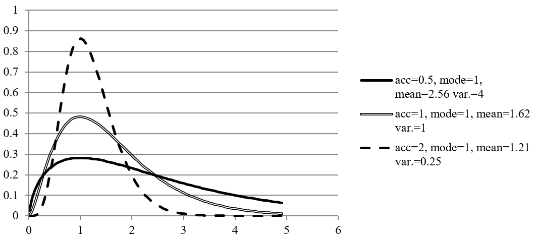
Figure 1: Gamma density graph for mode=1 and various standard deviations. “acc”=“mode/standard deviation”.
Let $i$ denote land use classes in CAPRI definition, whereas l and k are land uses in UNFCCC classification. Let $\text{LU}_{k}$ be total land use after transitions and $\text{LU}_{l}^{\text{initial}}$ be land use before transitions. Furthermore, let $T_{\text{lk}}$ denote the transition of land from use $l$ to use $k$. Noting that it is simpler and fully equivalent to maximize a sum of logged densities than a product of densities, the likelihood maximization problem can be written (with f being the gamma density function)
$${\max_{T_{\text{lk}}}{\log{\prod_{\text{lk}}^{}{f\left( T_{\text{lk}}|\alpha_{\text{lk}},\beta_{\text{lk}} \right)}}}}{= \max_{T_{\text{lk}}}{\sum_{\text{lk}}^{}{\log{f\left( T_{\text{lk}}|\alpha_{\text{lk}},\beta_{\text{lk}} \right)}}}}$$
$$\Rightarrow \max_{T_{\text{lk}}}\sum_{\text{lk}}^{}\left\lbrack \left( \alpha_{\text{lk}} - 1 \right)\log T_{\text{lk}} - \beta_{\text{lk}}T_{\text{lk}} \right\rbrack$$
subject to
$$\text{LU}_{k} - \sum_{l}^{}T_{\text{lk}} = 0 \; \left\lbrack \tau_{k} \right\rbrack$$
$$\text{LU}_{l}^{\text{initial}} - \sum_{k}^{}T_{\text{lk}} = 0\;\left\lbrack \tau_{l}^{\text{initial}} \right\rbrack$$
$$\text{LU}_{k} - \sum_{i}^{}{\text{shar}e_{\text{ki}}\text{LEV}L_{i}} = 0$$
The last equation is needed to convert land use in UNFCCC classification to land use in CAPRI classification, using a fixed linear transformation matrix $\text{shar}e_{\text{ki}}$. This discrepancy between land class accounts will be expanded on in a subsequent section. Forming the Lagrangian function and taking the derivatives with respect to land transitions gives the following first-order optimality conditions:
$$\ \left( \alpha_{\text{lk}} - 1 \right)T_{\text{lk}}^{- 1} - \beta_{\text{lk}} + \tau_{k}^{} + \tau_{l}^{\text{initial}} = 0$$
The parameters $\alpha$ and $\beta$ of the gamma density function were computed by assuming that (i) the observed transitions are the mode of the density, and (ii) the standard deviation equals the mode. Then the parameters are obtained by solving the following quadratic system:
$$\text{mode} = \frac{\alpha - 1}{\beta}$$
$$\text{variance} = \frac{\alpha}{\beta^{2}}$$
Annual transitions via Marcov chain in basic model
The implementation in CAPRI differs from the above general framework in that it explicitly identifies the annual transitions in year t $T_{\text{lk}}^{t}$ from the initial $\text{LU}_{l}^{\text{initial}}$ land use to the final land use $\text{LU}_{k}$. This is necessary to identify the annual carbon effects occurring only in the final year in order to add them to the current GHG emissions, say from mineral fertiliser application in the final simulation year. If the initial year is the base year = 2008 and projection is for 2030, then the carbon effects related to the change from the 2008 $\text{LU}_{l}^{\text{initial}}$ to the final land use $\text{LU}_{k}$ (=$T_{\text{lk}}$in the above notation, without time index) refer to a period of 22 years that cannot reasonably be aggregated with the “running” non-CO2 effects from the final year 2030. Furthermore the historical time series used to determine the mode of the gamma density for the transitions also refer to annual transitions.
Initially the problem to link total to annual transitions has been solved by assuming a linear time path from the initial to the final period, but this was criticised as being an inconsistent time path (by FW). Ultimately the time path has been computed therefore in the supply model in line with a static Markov chain with constant probabilities $P_{\text{lk}}$ such that both land use $\text{LU}_{l}^{t}$ as well as transitions $T_{\text{lk}}^{t}$ in absolute ha require a time index (e_luOverTime in supply_model.gms).
$$\text{LU}_{k}^{t} - \sum_{l}^{}{P_{\text{lk}}\text{LU}_{l}^{t - 1}} = 0\ ,\ t = \{ 1,\ldots s\}$$
Where $\text{LU}_{k}^{s}$ is the final land use in the simulation year s and $\text{LU}_{k}^{0} = \text{LU}_{k}^{\text{iniital}}$ is the initial land use. The transitions in ha in any year may be recovered from previous years land use and the annual (and constant) transition probabilities (e_LUCfromMatrix in supply_model.gms).
$$T_{\text{lk}}^{t} = P_{\text{lk}}*\text{LU}_{l}^{t - 1}$$
The absolute transitions may enter the carbon accounting (ignored here) and if we substitute the last period’s transitions we are back to the condition for consistent land balancing in the final period from above:
$$\text{LU}_{k}^{s} = \sum_{l}^{}{P_{\text{lk}}\text{LU}_{l}^{s - 1}} = \sum_{l}^{}T_{\text{lk}}^{s}$$
When using the transition probabilities in the consistency condition for initial land use we obtain
$$\text{LU}_{l}^{\text{initial}} - \sum_{k}^{}T_{\text{lk}}^{1} = 0$$
$$\Longleftrightarrow \text{LU}_{l}^{\text{initial}} = \sum_{k}^{}{P_{\text{lk}}^{}\text{LU}}_{l}^{\text{iniital}}$$
$$\Leftrightarrow 1 = \sum_{k}^{}P_{\text{lk}}$$
So the simple condition is that probabilities have to add up to one (e_addUpTransMatrix in supply_model.gms).
Annual transitions if SUPREMA is active
As the use of the Marcov-chain approach allows the annual transitions to be explicit model variables that could be used to compute annual carbon effects but leads to computational limitations especially in the market model a new approach was developed under SUPREMA (i.e. if %supremaSup% == on) by re-specifying the total land transitions as average transitions per year times the projection horizon and by considering for the remaining class without land use change (on the diagonal of the land transition matrix) only the annual carbon effects per ha, relevant for the case of gains via forest management.
The new accounting in the CAPRI global supply model may be explained as follows, starting from a calculation of the total GHG effects G over horizon h = t-s from total land transitions Llk and carbon effects per ha for the whole period elk:
$$G = Γ*h = \sum_{i,l}^{}{e_{\text{il}}^{}\text{L}}_{il}^{}$$
Where Γ collects the annual GHG effects that correspond to the total GHG effects divided by the time horizon G / h. These annual effects may be calculated as based on average annual transitions and annual effects for the remaining class as follows:
$$Γ= \sum_{i,l}^{}{e_{\text{il}}^{}\text{L}}_{il}^{}/h = \sum_{i≠l}^{}{e_{\text{il}}^{}\text{Λ}}_{il}^{} + \sum_{i}^{}{ε_{\text{ii}}^{}\text{L}}_{ii}^{} $$
Where Λil = Lil / h is the average land use change per year and εii is the annual carbon effect on a remaining class (relevant might be an annual increase due to growing forests while this will be zero for most effects based on IPCC default assumptions).
Using these average annual transitions for true (off-diagonal) LUC we may compute the final classes as follows:
$$ \text{LU}_{k,t} = \sum_{l}^{}{L_{\text{lk}}^{}\text{}}_{}^{} = \sum_{l≠k}^{}{Λ_{\text{lk}}^{}*h +\text{LU}_{kk}\text{}}_{}^{}$$
While adding up of shares (or probabilities) of LUC from class I to k over all receiving classes k continues to hold as stated above. It should be highlighted that the land use accounting implemented under SUPREMA avoids the need to explicitly trace the annual transitions in the form of a Markov chain and thereby economised on equations and variables.
Outer model – land supply
The outer problem is defined as a maximization of the sum of land rents minus a quadratic cost term, subject to the first order optimality conditions of the inner problem:
$$\max{\sum_{i}^{}{\text{LEV}L_{i}r_{i}} - \sum_{i}^{}{\text{LEV}L_{i}c_{i}} - \frac{1}{2}\sum_{\text{ij}}^{}{\text{LEV}L_{i}D_{\text{ij}}\text{LEV}L_{j}}}$$
subject to,
$$\text{LU}_{k} - \sum_{i}^{}{\text{shar}e_{\text{ki}}\text{LEV}L_{i}} = 0$$
$$\text{LU}_{k} - \sum_{l}^{}T_{\text{lk}} = 0\;\left\lbrack \tau_{k} \right\rbrack$$
$$\text{LU}_{l}^{\text{initial}} - \sum_{k}^{}T_{\text{lk}} = 0\;\left\lbrack \tau_{l}^{\text{initial}} \right\rbrack$$
$$\ \left( \alpha_{\text{lk}} - 1 \right)T_{\text{lk}}^{- 1} - \beta_{\text{lk}} + \tau_{k}^{} + \tau_{l}^{\text{initial}} = 0$$
The parameters of the inner model α and β may be determined as explained in the previous sections. For the outer model, we need to define the parameters c and D. We have a single data point of land use and land rent for each land use class. Since we have, for $N$ land classes, $N + N(N - 1)/2$ parameters, but only $N$ price-quantity pairs (one data point for each land class). This means that without any additional information, we could e.g. calibrate the model exactly by computing the c parameter, but have no information left for defining D. However, we have at our disposal prior estimates of the regional matrices of land supply elasticities that may be used to define prior densities for the elasticity matrix implied jointly by the c and D parameters and the inner problem. Another way of expressing this is that we compute a meta parameter matrix $\mathbf{\eta}\left( \mathbf{c},\mathbf{D},\mathbf{L}\mathbf{U}^{\text{initial}} \right)$ that is a function of the real parameters, and use the prior elasticity matrix as a prior for this meta parameter. If cast in this way, the problem becomes a Bayesian econometric estimation.
There are a few methodological and numerical challenges to overcome. In particular, we need to (i) analytically derive $\mathbf{\eta}\left( \mathbf{c},\mathbf{D},\mathbf{L}\mathbf{U}^{\text{initial}} \right)$, and (ii) ensure that the resulting model has the appropriate curvature to ensure a unique interior solution – anything else would result in a rather useless model. We start by simplifying the problem by observing that all the constraints (the first order conditions of the inner problem) can be replaced with an ordinary land constraint:
$$\sum_{i}^{}{\text{LEV}L_{i}} - \sum_{l}^{}{LU_{l}^{\text{initial}}} = 0$$
Note that the second sum is a constant. This simplification is based on the observation that the land transitions don’t appear in the objective function of the outer problem, so that all solutions to the inner problems are equivalent from the perspective of the outer problem, and that any land use vector that preserves the initial land endowment is a feasible solution to the inner problem.
Next, we formulate the first order condition (FOC) of the modified outer problem to obtain land use as an implicit function of the parameters, $F\left( LEVL,c,D,LU^{\text{initial}},r \right) = 0$. We can then use the implicit function theorem to compute the derivative of land supply $\text{LEV}L_{i}$ with respect to land rent $r_{j}$, which in turn can be used to define the elasticity matrix $\mathbf{\eta}$.
The first order conditions, and the implicit function, become
$$F\left( LEVL,\lambda,c,D,LU^{\text{initial}},r \right) = \begin{bmatrix} \frac{\partial\mathcal{L}}{\partial LEVL_{i}} = & r_{i} - c_{i} - \sum_{j}^{}{D_{\text{ij}}\text{LEV}L_{j}} - \lambda & = 0 \\ \frac{\partial\mathcal{L}}{\partial\lambda} = & \sum_{i}^{}{\text{LEV}L_{i}} - \sum_{l}^{}{LU_{l}^{\text{initial}}} & = 0 \\ \end{bmatrix}$$
In order to apply the implicit function theorem5) we need to differentiate the FOC once w.r.t. the variables $\text{LEV}L_{i}$ and $\lambda$ and once with respect to the parameter of interest, $r_{j}$, invert the former and take the negative of the matrix product. If (currently) irrelevant parameter are omitted, the following matrix of $(N + 1) \times (N + 1)$ is obtained (the “+1” is the uninteresting derivative of total land rent $\lambda$ with respect to individual land class rent $r_{i}$)
$$\left\lbrack \frac{\partial LEVL}{\partial r} \right\rbrack = - \left\lbrack D_{LEVL,\lambda}F(LEVL,\lambda,r) \right\rbrack^{- 1}D_{r}F(LEVL,\lambda,r)$$
$$\begin{bmatrix} \frac{\partial LEVL}{\partial r} \\ \frac{\partial\lambda}{\partial r} \\ \end{bmatrix} = - \begin{bmatrix} \frac{\partial F}{\partial LEVL} & \frac{\partial F}{\partial\lambda} \\ \end{bmatrix}\left\lbrack \frac{\partial F}{\partial r} \right\rbrack$$
Carrying out the differentiation specifically for land rent rj, we obtain:
$$\begin{bmatrix} \frac{\partial LEVL_{i}}{\partial r_{j}} \\ \frac{\partial\lambda}{\partial r_{j}} \\ \end{bmatrix} = - \begin{bmatrix} \left\lbrack {- D}_{\text{ij}} \right\rbrack & - 1 \\ - 1' & 0 \\ \end{bmatrix}^{- 1}\begin{bmatrix} I \\ 0 \\ \end{bmatrix}$$
Discarding the last row of the resulting $(N + 1) \times N$ matrix finally lets us compute the elasticity as
$$\left\lbrack \eta_{\text{ij}} \right\rbrack = \left\lbrack \frac{\partial LEVL_{i}}{\partial r_{j}} \right\rbrack\left\lbrack \frac{r_{j}}{\text{LEV}L_{i}} \right\rbrack$$
In the estimation, we assumed that the prior elasticity matrix is the mode of a density where each entry were independently distributed. Furthermore, the off-diagonal or any diagonal elements with negative priors were normally distributed, whereas the diagonal elements with positive priors (as required for a well-behaved curvature) were gamma distributed. For the standard deviation of elasticities we used either information from the prior estimates or some fall-back assumptions on standard deviations relative to the mode of elasticities. Denoting the prior elasticities with $e_{\text{ij}}$, we solved the following optimization problem, where parameters $\alpha$ and $\beta$ were already estimates as explained in the sections on the inner problem.
$$\max_{\eta,c,D}{\sum_{ij \in normal(i,j)}^{}{- {\frac{1}{s_{\text{ij}}^{2}}\left( \eta_{\text{ij}} - e_{\text{ij}}^{\text{jsa}} \right)}^{2}} + \sum_{ij \in gamma(i,j)}^{}\left\lbrack \left( \alpha_{\text{ij}} - 1 \right)\log\eta_{\text{ij}} - \beta_{\text{ij}}\eta_{\text{ij}} \right\rbrack}$$
subject to
$$\left\lbrack \frac{\partial LEVL_{i}}{\partial r_{j}} \right\rbrack = - \begin{bmatrix} \left\lbrack {- D}_{\text{ij}} \right\rbrack & - 1 \\ - 1' & 0 \\ \end{bmatrix}^{- 1}\begin{bmatrix} I \\ 0 \\ \end{bmatrix}$$
$$\left\lbrack \eta_{\text{ij}} \right\rbrack = \left\lbrack \frac{\partial LEVL_{i}}{\partial r_{j}} \right\rbrack\left\lbrack \frac{r_{j}}{\text{LEV}L_{i}} \right\rbrack$$
$$\begin{matrix} & r_{i} - c_{i} - \sum_{j}^{}{D_{\text{ij}}\text{LEV}L_{j}} - \lambda & = 0 \\ & \sum_{i}^{}{\text{LEV}L_{i}} - \sum_{l}^{}{LU_{l}^{\text{initial}}} & = 0 \\ \end{matrix}$$
and the curvature constraint using a stricter variant of the Cholesky factorization
$$D_{\text{ij}}\left( 1 - \delta I_{\text{ij}} \right) = \sum_{k}^{}{U_{\text{ki}}U_{\text{kj}}}$$
where $\delta$ is a small positive number and $I_{\text{ij}}$ entries of the identity matrix such that the factor $(1 - \delta I_{\text{ij}})$ shrinks the diagonal of the D-matrix, ensuring strict positive definiteness instead of semi-definiteness. We used $\delta = 0.05$. Furthermore, the Lagrange multiplier of the total land constraint, $\lambda$, was fixed at the weighted average of the rents $r_{i}$, i.e. $\lambda = \frac{\sum_{i}^{}{\text{LEV}L_{i}r_{i}}}{\sum_{i}^{}{\text{LEV}L_{i}}}$. Without the latter assumption, the parameters c and D are not uniquely identified.
Prior elasticities and area mappings
The empirical evidence obtained in the TRUSTEE project applied to prior elasticities for land categories based on Corine Land Cover (CLC) data. These categories are also covered in the CAPRI database based on various sources (see the database section in the CAPRI documentation):
The introduction has mentioned already three systems of area categories that need to be distinguished. The first one is the set of area aggregates with good coverage in statistics that has been investigated recently by JS Ay (2016), in the following “JSA”:
$$\text{LEVL} = \left\{ \text{ARAC},\ \text{FRUN},\ \text{GRAS},\ \text{FORE},\ \text{ARTIF},\text{OLND} \right\}$$
Where
ARAC = arable crops
FRUN = perennial crops
GRAS = permanent grassland
FORE = forest
ARTIF = artificial surfaces (settlements, traffic or industrial)
OLND = other land
The above categories are matching reasonably well with the definitions in JSA. A mismatch exists in the classification of paddy (part of ARAC in CAPRI but in the perennial group in JSA) and terrestrial wetlands (part of OLND in CAPRI and a separate category in JSA). Inland waters are considered exogenous in CAPRI and hence not included in the above set LEVL.
For carbon accounting we need to identify the six LU classes from IPCC recommendations and official UNFCCC reporting:
$$LU = \left\{ \text{CROP},\ \text{GRS}\text{LND},\ \text{FORE},\ \text{ARTIF},WETLND,RESLND \right\}$$
which is typically indexed below with “l” or “k” ∈ LU and where
CROP = crop land (= sum of arable crops and perennial crops)
GRSLND = grassland in IPCC definition (includes some shrub land and other “nature land”, hence GRSLND>GRAS)
WETLND = wetland (includes inland waters but also terrestrial wetlands)
RESLND = residual land is that part of OLND not allocated to grassland or wetland, hence RESLND<OLND
FORE = forest
ARTIF = artificial surfaces
In the CAPRI database, in particular for its technical base year, we have estimated an allocation of other land OLND into its components attributable to the UNFCCC classes GRSLND,WETLND, and RESLND:
$$\text{OLND}^{0} = {\text{OLND}G}^{0} + {\text{OLND}W}^{0} + {\text{OLND}R}^{0}$$
Lacking better options to make the link between sets LEVL (activity level aggregates) and LU (UNFCCC classes, technically in CAPRI code: set “LUclass”) we will assume that these shares are fixed and may estimate the “mixed” LU areas from activity level aggregates as follows
| GRSLND | = | GRAS + OLND · OLNDG0/OLND0 |
|---|---|---|
| WETLND | = | INLW + OLND · OLNDW0/OLND0 |
| RESLND | = | OLND · OLNDR0/OLND0 |
which means that the mapping from set LEVL to set LU only uses some fixed shares of LEVL areas that are mapped to a certain LU:
$$LU_k=\sum_i{\text{share}_{\text{i,k}}\text{LEVL}_i}$$
where 0 ≤ sharei,k ≤ 1.
Technical implementation
The key equations corresponding to the approach explained above are collected in file supply_model.gms or the included files supply/declare_calibration_models_for_luc.gms and supply/declare_calibration_models_for_land_supply.gms. The declarations of parameters, variables, equations, models and even some sets only used in the calibration given in these files are included by the “supply_model.gms” only if “BASELINE==ON” or if it was a CAPREG base year task that was carried out. Loading of priors, initialisation of parameters and variables for the calibration as well as the organisation of solve attempts are handled in new sections of file “cal_land_nests.gms”, in turn called by the gams file “prep_cal.gms”. This implies that the land supply and land use change calibrations were inserted before the ordinary calibration of the supply models.
SupremaSup should be active together with trustee_land to have smoother adjustments which may be set via the CAPRI GUI. In order to store the results of the calibration in a compact way that is compatible with the existing code, the existing parameter files “pmppar_XX.gdx” was used. The parameters of the land supply functions, called “c” and “D” above, were stored on two parameters “p_pmpCnstLandTypes” and “p_pmpQuadLandTypes”. As a new symbol (p_pmpCnstLandTypes) is introduced in an existing file, the first run of CAPRI after setting %trustee_land%==on may give errors if the file exists already but has been used with the previous land supply specification before. In this case it helps to delete or rename the old pmppar files.
At this point, it should also be explained that rents for non-agricultural land types were entirely based on assumptions (a certain ratio to agricultural rents). As there were no plans to run scenarios with modified non-agricultural rents, these land rents r used in calibration for those land types were subtracted from the “c-paramter”, so that it is implicitly stored in p_pmpCnstLandTypes and enters the objective function through the PMP terms. This requires changes if the rents shall be modified or if non-agricultural production shall be included in some simplified form.
Furthermore, the class Inland Waters (INLW) was given a special treatment: it is supposed to be entirely exogenous. For this purpose the special acronym “exogenousLandSupply” was introduced, and stored on the p_pmpCnstLandTypes and used to trigger an equation “e_exogenousLand “ in the supply model setting the variable to a constant. In that way, the fixity of INLW (or any land type, should it happen) is stored in the pmp terms and cannot be “forgotten”.
More detailed explanations on the technical implementation are covered elsewhere, for example in the “Training material” included in the EcAMPA-4 deliverable D5.
Concerning the improvements made under SUPREMA from a technical perspective, the changes are merged to the trunk. The approach is controlled by globals in capmod\set_global_variables.gms. If the global variable %supremaSup% == on, the yearly transition rate p_lucAnnualFac_sup is calculated. If it is %supremaSup% == off, the old approach using the Marcov chain is used with the respective variable v_luYearly. The FOC-approach to calculate LUC as described above is standard and independent from if the global variable supremaSup is on or off.
Emission Equations
Under EcAMPA 3 and partly in earlier projects (inter alia EcAMPA 2) new modelling outputs have been developed for indicators without matching reporting infrastructure helping users to organise the additional information. This applied for example to
1) Additional CAPRI results on land use results related to the complete area coverage, mappings to UNFCCC area categories and their transitions;
2) The carbon effects linked to these land transitions.
Furthermore, additional non-CO2 and CO2 related mitigation measures had been included under EcAMPA 3.
The scenarios including the emission equations are only run if %ghgabatement% == on, otherwise emissions are only calculated and not simulated.
The following emission equations have been implemented:
| Code | Description |
|---|---|
| GWPA | Agricultural emissions |
| CH4ENT | Methane emissions from enteric fermentation |
| CH4MAN | Methane emissions from manure management |
| CH4RIC | Methane emissions from rice production |
| N2OMAN | Direct nitrous oxide emissions stemming from manure management (only housing and storage) |
| N2OAPP | Direct nitrous oxide emissions stemming from manure application on soils except grazings per animal activity |
| N2OGRA | Direct nitrous oxide emissions stemming from manure managment on grazings |
| N2OSYN | Direct nitrous oxide emissions from anorganic fertilizer application |
| N2OCRO | Direct nitrous oxide emissions from crop residues |
| N2OAMM | Indirect nitrous oxide emissions from ammonia volatilisation |
| N2OLEA | Indirect nitrous oxide emissions from leaching |
| N2OHIS | Direct nitrous oxide emissions from cultivation of histosols |
| GLUC | Emissions related to indirect land use changes |
| CO2BIO | Carbon dioxide emissions from land use change due to losses of carbon in biomass and litter |
| CO2SOI | Carbon dioxide emissions from land use change due to soil carbon losses |
| CO2HIS CH4HIS | Carbon dioxide emissions from the cultivation of histosols Methane emissions from cultivation of histosols |
| CO2LIM CO2BUR | Carbon dioxide emissions from limestone and dolomit Carbon dioxide emissions from burning |
| CH4BUR | Methane emissions from burning |
| N2OBUR | Nitrous oxide emissions from burning |
| N2OSOI | N2O emissions from land use change due to soil carbon losses |
| GPRD | Emissions related to the production of non-agricultural inputs to agriculture |
| N2OPRD | Nitrous oxide emissions during fertilizer production |
| O2PRD | Carbon Dioxide emissions during fertilizer production |
Premium module
Overview
For the European Union, the CAPRI programming models cover in rich detail the different coupled and de-coupled subsidies of the so-called first Pillar 1 of the CAP, as well as major ones from Pillar 2 (i.e., Less Favoured Area support, agri-environmental measures, Natura 2000 support). The interaction between premium entitlements and eligible hectares for the Single Farm Payment (SFP) of the CAP is explicitly considered, as are the different national SFP implementations, possibly remaining coupled payments (previously under article 68 of Council Regulation (EC) No. 73/2009, from 2014 as “Voluntary Coupled Support”).
Decoupled payments – as with other premium schemes of the CAP from the present and past – are simulated in CAPRI relatively closely to their definition in existing legislation. The rather high dis-aggregation of the model template regarding production activities and the resolution by farm types inside of NUTS 2 regions clearly eases that task. Currently, 260 different voluntary coupled support schemes are implemented, in addition to decoupled income support (Basic Payment Scheme, BPS).
The payments – both in reality and in the model – tend to be defined in a cumulative manner. In 1992, the direct payments were introduced based on the previous price support levels multiplied by regional historic reference yields. The payments therefore became regionally differentiated. In the subsequent decoupling under Agenda 2000 and the following reforms, the single farm payments were defined based on the payments that each farm had previously received. The payments got very different expressed per hectare for farms in high yield regions versus low yield regions and for farms that had held animal payments versus arable farms. Then, the 2013 reforms introduced convergence of payment rates, both across farms (internal convergence) and between member states (external convergence). CAPRI reflects these incremental reforms, so that the payment rates in the most recent reform are based on coupled payments from MacSharry times.
Given that each reform has added complexity to the previous system, so too has the premium module of CAPRI grown to maintain the capacity to model previous reforms while allowing novel features such as greening to be introduced. Nevertheless, two generic features can be distinguished, that form the basis for many payments: the basic concept of a premium payment, and the idea of payment entitlements. Those are treated in separate sections here. Then, we proceed to describe the incremental reforms of the first pillar of the CAP, starting with the most recent, and the implementation of selected second pillar payments. Finally, we discuss certain elements relating to the reporting of premium payments, most notably the financing over different budgets.
Basic concept
In the CAPRI supply module, premiums are always paid per activity level (per hectare or per animal) basis. They can be differentiated by the low and high yield variant of each crop activity. The premiums are calculated in the premium module from different premium schemes.
A premium scheme (such as DPGRCU for the Grandes Cultures premiums after the Fischler reform) is a logical entity which encompasses:
- A specific application type (defining the basis for the payment amount)
- a region or regional aggregate to which it is applied,
- Possible ceilings in entitlements (CEILLEV) and in value (CEILVAL)
- Payment rates for possibly several lists of activities (such as PGGRCU for all types of Grandes Cultures or PGPROT for protein crops).
- Optionally an indication of the marginal payment when a ceiling is reached
- Optionally a modifier for different amounts per technology
The schemes provide many-to-many mappings between policy instruments and agricultural activities: each scheme can apply to many different activities – with possibly differentiated rates – and each activity can draw support from different schemes.
The application type defines how the nominal amount (called PRMR) is applied. Currently, the following application types are supported:
- perLevl = per ha or head
- perSlgtHd = per slaughtered head
- perYield = per unit of main output
- perHistY = per historic yield
- perLiveStockUnit = per livestock unit
- noDirPay = Norwegian direct payment
- noPriceSup = Norwegian price support
The application type points to a factor by which the nominal amount PRMR (for PRemiuM in Regulation) is converted to a declared value per hectare or head (PRMD). For perLevl, the factor is unity (it is already per hectare), but for instance for perYield, the amount is interpreted as a payment per unit of main output. That is used for the Nordic Aid Scheme for dairy cows in the northmost parts of Europe and for coupled payments in Norway.
Each payment is defined for one or seveal groups of activities, functioning as lists of eligible activities. Additionally, the payment can be applied in different rates to the high and low yield variant, to model e.g. an extensification premium.
Each premium scheme also has up to two ceiling values:
- ceilLev = Ceiling on LEVL, i.e. the number of hectares or heads
- ceilVal = Ceiling on the total budget (envelope) spent on the scheme
In the basic setting, the ceilings work as the old Grandes Cultures payment: if the total quantity (hectares or amount) exceeds the ceiling, then the payment to each farmer is reduced so that the ceilings are respected. This means that the marginal payment is somewhat reduced but does not become zero. For some other schemes, such as the Basic Payment Scheme of the CAP 2014-2020, there is a hard limit on the number of payment entitlements, so that the marginal payment becomes zero if the ceiling is overshot. That behaviour can be triggered by including the payment scheme set element in a special set PSDPAY_cutEndog, as in the following example from “pol_input/mtr_until2013.gms”.
PSDPAY_cutEndog(“DPSAPS”) = YES;
PSDPAY_cutEndog(“DPREG”) = YES;
PSDPAY_cutEndog(“DPFRMS”) = YES;
PSDPAY_cutEndog(“DPFRMF”) = YES;
PSDPAY_cutEndog(“DPGREEN”) = YES;
The following figure shows the technical implementation at an example:
Figure 14: Example of technical implementation of a premium scheme

The sets of payments, exemplified by DPGRCU in the figure, and the activity groups, exemplified by PGGRCU and PGPROT are defined in the file policy/policy_sets.gms. Since this is a “static” GAMS file used in any simulation, it contains the gross list of all policies that currently can be simulated, including legacy ones. In order to work efficiently with the acronyms which define the application types, these are converted to numerical attributes as shown below (‘policy/policy.gms’):

CAPRI also provides the possibility to incentivise extensification or intensification via the payments. Most production activities come in technological variants, by default one higher yielding and one lower yielding one, and those variants can be eligible to different rates of premium payments. This is used for instance in the implementation of agri-environmental schemes in the file policy/rd_logic.gms as shown in the figure below. The parameter p_technFact is the standard coefficient that modifies the technology of the production activities in CAPRI. In the figure below, the two statements change the rate of premium payments for the set of currently active regions (rs), for all model activities (MPACT), for all agri-environmental schemes (psdpay_ae) with different rates for technology T1 (high yield) and T2 (low yield) in the case where T2 exists. +0.5 for T2 means that the premium payment in the model becomes the nominal rate times (1 + 0.5), i.e. 50% higher, whereas the -0.5 for T1 means that the premium payment in the model becomes the nominal rate times (1 – 0.5), i.e. 50% lower. This approximates the stylized fact that agri-environmental schemes, which in reality consist of a wide range of measures, in general favour extensive technologies (see section on Pillar II payments below).

The general flow of logic inside of CAPRI (inside the model file capmod.gms) as regards premiums is shown in the following figure. The process starts by loading baseline data, including calibrated behavioural parameters. That data set represents an equilibrium situation for the policy (premiums) that were used in the baseline generation process.
After loading data, the file with declarations of all available premium schemes et cetera (policy_sets.gms) is loaded. The particular policy to use in the present simulation is contained in the policy file with the name defined by the placeholder (environment/macro variable) %result_type%. This string will also be part of the file name used for the simulation results.
The premiums defined in the policy file is processed by the file policy.gms. That processing implies a translation of the regulation-like definitions used in the policy file to parameters useful for CAPRI.
Within the simulation algorithm itself, a special file called prmcut.gms is called repeatedly, with the purpose to cut effective premium rates paid in case any ceiling is overshot, so that budgets are respected.
Figure 15: General flow of logic of CAPRI model as regards premiums

Generally, all attributes for a premium scheme are mapped down in space, e.g. from EU27 to EU 27 member states, from countries to NUTS1 regions inside the country, from there to the NUTS2 regions inside the NUTS1, and from NUTS2 regions to the farm types in a NUTS2 region (see ‘policy/policy.gms’), e.g.

In order to map the premium rate as defined in a legal text into one paid out on a per-activity basis, the relevant activity based attribute matching the application type is set to a premium modification factor (“Ap_premModfFactT”) as shown below:

The actually declared premium per activity unit (ha, [1000] [slaughtered] heads) is then the multiplication of the premium rate and that modification factor. For crops, the unit of the resulting entries are current € per ha, for animal, it depends on the exact definition of the activity level (per [1000] [slaughtered] heads).

These declared rates can hence be aggregated to higher regional units using the activity levels as weights, e.g. from farm types to NUTS2:

Before the supply module is started between iterations, the current activity levels and premiums paid out are summed up for each scheme and regional level where ceilings in levels or value are defined. If one of the aggregated sums exceeds the ceilings, all premium rates for the scheme are cut proportionally to fit under the tighter of the two envelops:

From the declared rates and these cut factors, the actually paid premiums are defined:

The indivudal premiums from each premium scheme are then added up to arrive at one average rate for each activity which enters the objective function of the supply model, the data base and post-model reporting:

An example of a payment with a ceiling
We explain the different elements and steps in the following based on an example of the slaughter premium for adult cattle of 80 EURO per slaughtered head in Latvia, defined in 2004. The following screen shot comes from the policy file gams/pol_input/mtr_until2013.gms, with some lines hidden.

- The application type defines the criterion upon which the payment depends, in the case of the slaughter premium it is defined per slaughtered head.
- The regulation premium rate (PRMR) is the default (maximum, uncut) amount of the premium according to regulatory texts, for all activities coverd by the premium group (here PGMEAT) and regions for which the premium is defined. In the example, this means that it is 80 EURO for the group of activities PGMEAT, which is dairy cows, suckler cows, male adult cattle and fattened heifers, in Latvia (LV000000). This is defined in a hierarchical way: if it is set to 80 EURO for the EU and not set at all at lower regional level, the 80 EURO are mapped down to all sub regions by the program. The program also lets you define groups of activities that are linked to the premium. In this case a group PGMEAT has been defined which contains the relevant animals (set s_PSGRP(*) in the file ‘policy_sets.gms’).
- The declared amount in the activity definition of CAPRI (per ha, per head, per 1000 heads) way that the amount PRMR should be applied or declared in CAPRI is called declared premium (PRMD) and applies per head or hectare. In our example, the regulation says that 80 EURO should be paid when the animal is slaughtered. That means that in order to get the amount per living animal and year, the 80 EUROs have to be multiplied by the frequency with which the animal is slaughtered. For male beef cattle it is 1/year whereas it for dairy cows is something like 1/5 years. These numbers come from the CAPRI database.
- Regional ceiling, expressed in maximum number of premiums paid and/or total payment in EURO. In the example with the slaughter premiums, this is used to set a national ceiling limiting the total amount spent on slaughter premiums to 9.946 million euro. There can be additional ceilings at other regional levels, and the most strongly binding is always the one that limits payments.
Those four pieces of information are generally easily accessible without further processing from the regulatory texts. Starting with PRMR and APPTYPE (information pieces 1 and 2 above), it is possible to calculate (3), PRMD, the amount of premium per head or hectare that would be paid if there were no (active) ceiling. These preparatory calculations, e.g. the hierarchical break down from higher to lower regional level and from activity groups to individual activities, as well as the calculations of PRMD from PRMR (using APPTYPE) is carried out in a file called ‘policy/policy.gms’ as shown above.
For most premiums in CAP there are ceilings, which if they are binding decrease the average amount of premiums actually paid (effective premium, PRME) per head or hectare. As discussed, due to the different kind of ceilings, the reduction of premiums and the treatment of PRME can only be done endogenously during the simulations depending on the simuled production patterns.
How is this problem solved in CAPRI? The effective premium (PRME) is exogenous during the optimisation of the supply model6), but adjusted iteratively between the main model iterations. So, for most premium schemes, the premium level is constant in the objective function and hence the model does not realise that the marginal premium payment is zero as soon as the ceiling is reached. Technically, the iterative adjustment of the effective premiums PRME is handled in a file called ‘policy/premcut.gms’ for “premium cut”. That reasoning is correct as long as the ceiling is not farm specific.
In each iteration, once all regional model are solved, the program adds up total number of premium units (hectares or heads for which it is paid) that belong to each ceiling. In most cases this simply means summing up number of animals or hectares of the activities for which each premium applies. This is also multiplied with the declared amount PRMD to get the total payment which would be paid if it would not be cut. For each premium this is compared to the ceilings defined (total level with the level ceiling and total amount with the value ceiling) and a “cut factor” is calculated, which defines how much the premium has to be reduced in order to fit under all ceilings. Then PRMD is multiplied by this factor to get the effective premium (PRME) for the next iteration.
Pillar I
The MTR-reform and the health check
On 26 June 2003, EU farm ministers adopted a further fundamental reform of the Common Agricultural Policy (CAP). The central element of the 2003 CAP reform was the introduction of the so-called single payment scheme (SPS). The SPS is based on payments entitlements linked to eligible land, but decoupled from production. However, to avoid abandonment of production, Member States could still choose to maintain a limited link between subsidy and production under well defined conditions and within clear limits. Moreover, these new “single farm payments” would be linked to environmental, food safety and animal welfare standards and obligations.
Key elements of the 2003 CAP reform were:
- A single farm payment for EU farmers, independent from production; limited coupled elements may be maintained to avoid abandonment of production;
- land receiving payments should be kept in good agricultural and environmental condition (G.A.E.C). “Good agricultural condition is generally interpreted to mean that the land will not be abandoned and environmental problems such as erosion will be avoided” this requirement could be interpreted as re-establishing the link between the payment and the factors of production employed (land management practices) and ultimately current production; some form of management of the land should be maintained;
- entitlements are tradable within the EU member states (not among them) but certain limitations are imposed (Ciaian, Kancs and Swinnen, 2010). For example, in the Netherlands, entitlements can be transferred among farmers only when the farmer has land without entitlements;
- areas already under permanent pasture should must remain so; in practise, certain reductions at regional level were accepted before Member States would be forced to interact.
- a strengthened rural development policy based on expanded EU budget outlayswith more EU money, new measures to promote the environment, quality and animal welfare and to help farmers to meet EU production standards starting in 2005,
- a reduction in direct payments (“modulation”) for bigger farms to contribute to finance the new rural development policy,
- a mechanism for financial discipline to ensure that the farm budget fixed until 2013 is not overshot,
- revisions to the market policy of the CAP:
- asymmetric price cuts in the milk sector: The intervention price for butter will be reduced by 25% over four years, which is an additional price cut of 10% compared to Agenda 2000, for skimmed milk powder a 15% reduction over three years, as agreed in Agenda 2000, is retained,
- reduction of the monthly increments in the cereals sector by half, the current intervention price will be maintained,
- reforms in the rice, durum wheat, nuts, starch potatoes and dried fodder sectors.
In implementing the SPS, member states (MS) could opt for a historical model (payment entitlements based on individual historical reference amounts per farmer), a regional model (flat rate payment entitlements based on amounts received by farmers in a region in the reference period) or a hybrid model (mix of the two approaches, either in a static or in a dynamic manner). An overview of the implementation of direct payments under the CAP in the different MS can be found at http://ec.europa.eu/agriculture/markets/sfp/ms_en.pdf.
Denmark, Germany, Luxembourg, Finland, Sweden, England and Northern Ireland applied a hybrid model. The remaining MS implemented the historical model. From 2007 onwards, dairy payments will be decoupled from production and included in the single payment scheme in all MS.
Although the intention of the CAP reform 2003 is to decouple payments, some payments were not included. In particular the crop specific payment for protein crops, 60% of the payment for starch potatoes, 42% of the payment for rice, the quality premium for wheat and the area payment for nuts. Market organizations for commodities not included in the reform also remained in place. For sugar this changed by the end of 2005 as a reform of the sugar market was decided upon by the EU ministers of Agriculture. The reform included a reduction of the administrative price levels of sugar and sugar beet by with 36%, the introduction of a compensation payment for sugar beet farmers, a premium scheme for the termination of sugar production at factory level (what is referred to as the 'restructuring scheme') and the opportunity to purchase quota sugar. The compensation for sugar beet farmers will be included in the single payment scheme.
Until the end of 2007 for several fresh and processed fruit and vegetables coupled payments were given. Since 2008 fruit and vegetables are decoupled and land covered by fruit and vegetables is eligible for payment entitlements under the decoupled aid scheme which applies in other farm sectors (EC, 2007). All existing support for processed fruit and vegetables will be decoupled and the national budgetary ceilings for the SPS will be increased accordingly.
The last step of the EU CAP reform dates from 20 November 2008 when EU agriculture ministers reached a political agreement on the so-called Health Check (HC) of the CAP. Among a range of measures, the agreement abolishes arable set-aside, increases milk quotas gradually leading up to their abolition in 2015, and converts market intervention into a genuine safety net (EC, 2009). Ministers also agreed to increase modulation, whereby direct payments to farmers under the SPS are reduced and the money transferred to the Rural Development Fund. This should allow a better response to the new challenges and opportunities faced by European agriculture, including climate change, the need for better water management, the protection of biodiversity, and the production of green energy. Member States will also be able to assist dairy farmers in sensitive regions to adjust to the new market situation.
Under the HC of the CAP it was decided that remaining coupled payments should be decoupled and moved into the Single Payment Scheme (SPS), with the exception of suckler cow, where Member States may maintain current levels of coupled support. Moreover, member states are allowed to review the decision taken on the decoupling of fruit and vegetables in 2007, provided that it results in lower coupled payments. For soft fruits transitional support will continue until 31st December 2011 and be converted into decoupled payment as of 2012 (EC, 2009). Before the HC Member States could retain by sector 10 percent of their national budget ceilings for direct payments for use for environmental measures or improving the quality and marketing of products in that sector (Article 68/69' measures: Assistance to sectors with special problems). Under the HC this possibility will become more flexible. The money will no longer have to be used in the same sector; it may be used to help farmers producing milk, beef, goat and sheep meat and rice in disadvantaged regions or vulnerable types of farming; it may also be used to support risk management measures such as insurance schemes for natural disasters and mutual funds for animal diseases; and countries operating the Single Area Payment Scheme (SAPS) system will become eligible for the scheme (EC, 2009).
Money for Article 68/69’ measures increases as currently unspent money can be used for these measures as well. The Rural Development budget money increases as money shifted away from direct aid based on expanding (modulation) increases to 10% of the direct aid. The additional funding for Rural Development obtained this way may be used by Member States to reinforce programs in the fields of climate change, renewable energy, water management, biodiversity, innovation linked to the previous four points and for accompanying measures in the dairy sector. This transferred money will be co-financed by the EU at a rate of 75 percent and 90 percent in convergence regions where average GDP is lower. Finally for our purposes it is important to mention that under the HC of the CAP a series of small support schemes will be decoupled and shifted to the SPS from 2012. The energy crop premium will be abolished.
In CAPRI, The different implementations of the single farm premium (SFP) introduced with the so-called Mid Term Review of the CAP apply the same logic as for the payment schemes. To give an example, the regional implementation is called DPREG, and might have different payment rates for arable crops (PGARAB) and grass lands (PGGRAS).
The general way these premiums are introduced in CAPRI is shown below. From a reference situation (expost statistical data) and the premiums valid at that time, it is first determined (Decision D1) how much of each existing payments in each scheme are continued to be payed as a coupled scheme, and how much is going into envelops for different types of decoupled payments (part of decision D2). That envelop can be at farm, regional or Member State level and can be implemented in different ways (e.g. historic implementation, regional, regional with different payment rates to arable or grass lands).
Figure 16: General way of SFP implementation in CAPRI

In opposite to the reforms until Agenda 2000, there are hence in most cases not longer premium rates or individual ceilings in hectares found in legal texts. Rather, these are calculated by the model itself from the decoupled part of the “old” Mac Sharry and Agenda 2000 premiums which introduces additional complexity in the model code.
Only an overall budget envelop is given covering all pillar I premiums of the EU CAP (“old” MacSharry and Agenda 2000 premiums, SPS premiums, article 63/68/69 premiums, etc.) per Member State nad per year on the position p_premDataE(MS,SIMY,“DPMTR”,“CEILVAL”) in ‘pol_input/mtr_hc.gms’. Here MS refers to member states and SIMY to a certain year.
Single area payment scheme (SAPS)
The MS who joined the EU since 2004 could choose to apply the single area payment scheme (SAPS), a simplified area payment system, for a transitory period until end 2010 or to apply the same system as in the EU-15 immediately. The most important difference between the SPS and the SAPS is that the entitlements under the SPS can be transferred between farms.
From a technical viewpoint, the single-area premium scheme (SAPS) is the easiest to implement:

As it defines a flat rate premiums per ha of agricultural land. The ceilings in values and thus the application rates per ha are step wise increased over time:

To reach their full level in 2013 (EU 10) or 2016 (Bulgaria and Romania).
During that transition period where not yet the full EU premiums were paid out, the Member States had the right to paid up to certain limits to so-called complementary national direct payments (the list of schemes used in CAPRI was shown above). They also edited in a tabular format:

These top-ups have to be reduced towards the end of the period where the the Pillar I premiums are phased in:

Non-SAPS implementation
The non-SAPS implementation of the Mid-Term Review package is far more demanding. First of all, the countries could, at least in the earlier years of the reform, keep certain percentages of specific premium scheme still coupled to production. These coupling factors are stored on the parameter p_couplPercent_E:

The amount of payments which is not kept coupled is then paid out to different implementations of the MTR:
- Regional implementation where all arable crops (PGARAB)

- And permanent grass land (PGGRAS) is eligble

- The historic implementation

The exact set member ship depends on the year. The distribution shares which map the decoupled part of the premiums received under the Agenda package (see above) to these implementation schemes are edited on the Table “p_premToDDTarget_E”

That information is the basis to define regional premium envelops (= CEILVAL) for the different Member states. That is a rather complex program (‘policy/calc_mtr.gms’). A first key statement defines the remaining budget envelops for the still coupled payments. It takes the minimum of the existing ceiling values for that scheme (CEILVAL) or the total payments paid out times the modulation factors and multiplies it with the coupling degree.

There two other factors:
- A possible greening share according to the October 2011 proposal by the Commission, see the section on CAP 2014-2020 for more details
- A national ceiling cut factor which aligns the envelops calculated from the past payments with he total MTR ceiling as defined in the legal texts.
The part which is not longer coupled goes into the decoupled schemes:

The total budget for the new MTR schemes is derived from the summation of all the old Agenda premiums. The total payments under a scheme such as the Grandes Cultures schemes are corrected for any possible remaining coupled payments:

After that, a possible share going into the greening payment (from 2014) is deducted:

And, finally, a factor is applied which lines up the total historic payments as defined from the CAPRI data and premium schemes in that Member State with the total MTR envelop:

That sum if then distributed to the relevant MTR implementation scheme according to the distribution keys defined above:

These calculation require that first the total premiums received in the history period are calculated which is done in ‘policy/calc_mtr_top.gms’.
CAP 2014-2020
From 2014 onwards, a new agricultural policy entered into force. The key elements of the policy were (i) convergence of payment rates between member states and farmers within member states, (ii) the expansion of the option to use coupled support beyond the previous articles 68/69, and (iii) the introduction of three “greening requirements”. These elements were introduced into CAPRI, and their use can be inspected in the commonly used baseline policy file “gams/pol_input/cap_after_2014/ref.gms”, the entire content of which is shown below:

Since the mechanisms behind each of the three elements is somewhat complex, the file relies on include files to define each of the three components. The include files are stored in the scenario directory (gams/scen) of the CAPRI system, and which particular include files to use is indicated by the string variables ($setGlobal) in the first three code lines. The actual logic of the policy file, also the inclusion of the indicated three files, takes place in the file included in the final line, referred to as the base scenario file.
Convergence between member states is set by adjusting the total budget of the CAP first pillar. Regarding the convergence of payment values per entitlement (IUVs, for Individual Unit Values) inside countries, the regulation allows ample room for national customization. Countries define the regions within which convergence occurs, the end year by which convergence shall be achieved, any remaining maximum span for the IUVs after convergence, and the mathematical formula to use for reducing high IUVs and increasing low ones. The file gams/scen/premiums/bps_convergence.gms defines the options chosen by member states in 2014.

Two different uses of the convergence mechanism are illustrated by Austria and Greece, which apply very different models. Austria applies the full convergence using a linear model over time, with the same target payment rate in all of Austria. The convergence should be complete in 2019. This is obtained by assigning all Austrian regions to one generic “BPS-region”, for convenience the first one, called “rbps1”. Since the convergence mechanism later on works per member state, it is no problem that rbps1 is also used for e.g. the Netherlands. Then, the convergence option is set to “bps_linear” and the target year to 2019. Finally, the two parameters defining the rate of the final convergence are set, or, if you like, the width at the end of the convergence funnel and the handling of payments outside of that funnel. For Austria, the parameters are both set to “1”, which means that all farms will get exactly the same payments per hectare after convergence is complete in 2019.

Greece applies different models for different types of regions, depending on the character of agriculture in the region. We approximate this in CAPRI by classifying the NUTS2-regions according to the shares of arable land, grass land and permanent crops in a historical year (2008). Based on those shares, three BPS-regions are created, within each of which the same convergence model is applied. The convergence is linear, but with the additional 30-percent-rule applied, defining that no farm (supply model region) should get more than 30 percent higher payments per hectare than the average of the BPS-region. Convergence proceeds up to the year 2019, and in each year, the lower limit for convergence, expressed as a share of the averge of the BPS-region, is set to 90%. The lower limit defines whether a farm needs convergence or not. Farms above the lower limit will get the same payments per unit as before, but for farms below the limit, the final option “p_bps_tunnel_gap_closure” kicks in, and defines what share of the gap to the lower convergence limit should be closed. For Greece, this value is set to 1/3, implying that for a farm receiving less than 90% of the average payment in the BPS-region, 1/3 of the gap shall be closed. The increased premiums are financed by a linear reduction of the payments to all farms with payments above the average payment, while also capping the highest premiums to be no more than 30% higher than the regional average.

The code implementing the logic behind these various settings is generic and found in the file “gams/policy/implement_bps.gms”. The result is a payment per region, defined using the general premium mechanism of CAPRI, that is called “dp_bps” and with the eligible activity list “pgsaps”. The application type is “perLevl” and the budget is set on national level in the base scenario file “gams/scen/base_scenarios/cap_2014_2020.gms”.
Voluntary Coupled Support is defined using the standard premium mechanisms of CAPRI, based on notifications received from the European Commission. We have interpreted the notified target activities in terms of CAPRI activities, and set budget ceilings and nominal amounts in the file “gams/scen/premiums/coupling/cap_2013_2020_vcs.gms”.
The Greening Measures can be steered by the modeller. Even though the greening in itself is complex in implementation, the choices open to the CAPRI modeller are limited. The standard greening policy switches can be inspected in the file “gams/scen/premiums/greening/cap_2013_2020_greening.gms”:

The first statement defines the share of the national pillar 1 envelope that is dedicated to the “greening top-up”. By default, this is 30%. Then, a set of active greening measures is populated. There are three options available, and by default, they are all active:
- The share of permanent grass land to arable land cannot decline relative to the base year.
- A minimum measure of crop-diversity must be maintained.
- A share of land must be allocated to certain activities counting as “ecological set-aside”.
The shares of activities eligible as ecological set-aside is then defined in the concluding parameter definition in the file. The set-aside rate itself is defined as a string variable “$setglobal greening_setasiderate 5”, defining it to be 5% by default. The three greening restrictions are implemented as constraints in the supply models. The greening top-up is implemented as a standard CAPRI premium called DPGREEN. The logic behind the greening restrictions is activated in the include file “policy/define_greening_limits.gms”.
The CAP 2014-2020 also contains three more payment schemes: Support to young farmers, support to smaller farms (first hectares) and support to areas with natural constraints (ANC). These payment schemes, with their associated budgets, are defined in the base scenario file.
The following figure summarizes the logic of the CAP 2014-2020 reference policy as implemented in the CAPRI policy module in the policy file pol_input/cap_after_20147ref.gms.
Figure 17: The logic of the CAP 2014-2020 reference policy as implemented in the CAPRI policy module

Tradable Single Premium Scheme entitlements
With the so-called Mid Term Review of the Common Agricultural Policy, the so-called Single Farm Premium (SFP) as a decoupled payment was introduced which is implemented as a subsidy which does not require production, is subject to cross-compliance and paid per ha up to a number of entitlements. The original entitlements, defined on a hectare basis, had been distributed to farmers operating the land and not the land owners. Both land and entitlements can be traded independently from each other. After a sequence of reform steps, basically all crop production sectors are now included in the subsidy program, so that farmers can be assumed to have received entitlements for all hectares they cropped historically. The same was true from the beginning for the so-called regional implementation. If the land available to agriculture decreases, e.g. by urbanization, some entitlements cannot not longer be matched with a hectare of eligible land. Such unused entitlements are removed from the markets after a number of years.
In CAPRI, the assumption in the baseline is that all hectares used by agriculture are able to claim the SFP and that any unused entitlements had been removed so that the SFP becomes fully capitalized into land. Subsequent changes in the premiums including the SFP, prices or other policy instruments in a counterfactual run could decrease the marginal returns to agricultural land. Based on the land supply curve implemented in CAPRI, agricultural land use would shrink and some entitlements become unused. Vice versa, if changes let the marginal return to land increase, the entitlements become the limiting factor to claim the subsidy. The increase is thus mapped into an economic rent to the entitlement. If changes generate rents on entitlements in some farm types and not in others, one would assume that trade in entitlements will occur. A simple algorithm to trade the entitlement is now included in CAPRI and described below.
Switching on the entitlement trade
The trade module is implemented in the file ‘policy/prem_entl_trade.gms’ which is included on demand in capmod and called in each iteration

By default, the entitlement trade is switched OFF in the general settings file of CAPMOD, called gams/capmod/set_global_variables.gms

The basic idea of the module is very simple: shift entitlements from farm type or regions which unused entitlements to other farm types or regions which have an economic rent on their entitlements. The trading entities should receive the very same premium on the entitlement for the current implementation in the code. One should hence set the trade level according to the regional level for which flat rate premiums are implemented as shown below in an example:

How the entitlement trade works
The following code pieces are taken from ‘policy/prem_entl_trade.gms’. In a first step, the demand of entitlements is determined. The dual value does only provide an indication that entitlements are scarce, but not how many additional entitlements are needed. Accordingly, first, the average marginal value of the different type of entitlements is determined:

From these a maximum of 10% is defined as the demand in each iteration:

In order to take differences in the marginal returns into account, an indicator based on the squared value is used:

It serves as the distribution key of unused entitlements, which are determined as follows:

Next, the number of unused entitlements is stored:

As seen, only 50% of the unused entitlements are released in any iteration. We next determine the size of the markets, i.e. total demand and supply:

The supply is then distributed according to the squared value of the individual demanders

An example printout
The following code snippet shows an example for a NUTS2 regions and the related farm types for a test run for Greece without the market module:

As seen from above, we have two farm types in the starting situation which acts as demanders, i.e. have a marginal value on their entitlements (016 and 999). Their marginal value on the entitlement is quite high in the starting situation with > 125 € / entitlement. We have also a total of 3639 ha after the first round of unused entitlements which can be sold to the demanders. Distributing half of them (ca. 1800 ha) to the two demanders reduces the marginal value of the entitlements already below 95€, the next round distributed ca. 900 ha and brings the price down to 50€ until in the last round almost nothing is left for distribution and the value of the entitlements has dropped below 10€. The reader should note the trade is not yet taking into account in the income calculation of the farm types.
Finally, we come to the main point which motivated the introduction of that module. As indicated above, we interpret the SFP as a subsidy to agricultural land use which at the margin is capitalized in the land rent. It thus increases the marginal returns to land use in agriculture. In our baseline, we start with a situation with an assumed equilibrium in land markets, i.e. marginal returns in agriculture including any subsidies are equal to marginal returns of alternative uses.
Reducing the SFP will render agricultural land use less competitive so that land owner will rent out less to agriculture and put the land into other uses. That effect can be clearly seen below in the first iteration: in the farm types where the SFP drops due to uniform SFP at NUTS2 in Greece, land use is reduced. Total land use in Greece drops by 1.2%. But if we re-distribute the subsidy between farm types, farms which were competing before with below average subsidies against alternative land use possibilities now would like to expand land use. Without additional entitlements, they cannot: the marginal return on the next ha drops by the SFP rate. But once they buy entitlements, they offset a larger part of the land loss: in step twp, the reduction is only about 0.6%. And towards the end, the basically a no-change in land use, as we would have assumed at the aggregated level if the same type of subsidy is paid on average with the same rate.
Pillar II
Overview
Modelling of Pillar II for an EU-wide assessment provides a specific challenge given data availability regarding measures which are programmed and implemented at Member State or even regional level. Official reporting of measures under Pillar II in standardized data bases uses a rather rough categorisation, so are e.g. all agri-environmental measures grouped into one category. But even at that rather aggregated level, there is no ready to use data base available to researchers, especially with a regional resolution. A first task therefore consisted in building up a suitable data base on funds for Rural Development measures, a task undertaken by a team which had already compiled such data in the past (BALDOCK et.al. 2002).
The most important measures from a budgetary view point are the Agri-Environmental Schemes and the Less Favourite Area Payments. Therefore some care must be taken to model these measures accurately. The project draws here on the work of a study by LEI and IEEP (LEI and IEEP 2009) for DG-AGRI, which use in the case of the agri-environmental payments analysis based on FADN and for LFA based on FADN and CLUE (Verburg et.al. 2010) results.
Table 26: Overview of pillar II measures modelled in CAPRI
| Measure type | Measure codes EU | Modelling approach in CAPRI |
| LFAs | 211-212 | Regional direct support. Distribution over sectors and regions based on FADN data and CLUE results. |
| Natura 2000 | 213,224 | Regional direct support. Distribution over sectors and regions based on FADN data and CLUE results. Conditional on extensive technology being used. |
| Agri-environment | 214-215 | Regional direct support. Distribution over sectors and regions based on FADN data. 50% of the support directed towards TF8 farm types 1, 2, 3, 4 and 8 is conditional on extensive technology being used, for remaining amounts extensive as well as intensive technology is eligible. |
Modelling of LFA
The LFA measure was implemented as a direct payment to cropping and grassland, with the same amount for all cropping activities except for fallow land. The first challenge encountered when implementing the LFA premiums is that the regions do not coincide with the administrative regions used in CAPRI. – Recall that CAPRI only has one single representative firm in each nuts 2 region (or up to nine farm types). In reality, thus, only a share, generally much less than 100%, of the land in a nuts region is eligible for LFA payments, and it may very well be the case that the agricultural production on that land is different from the regional average. For example, one may expect that a mountainous LFA area contains more grass land than the surrounding flat land agricultural areas in the same nuts 2 region. In order to capture a possible bias of this nature, a GIS tool (CLUE-model) was used to compute the shares \(S_{ij}\) of LFA in different broad land use classes j \(\in\) {non-irrigated arable land, irrigated arable land, pasture, permanent crops} in each region i. Those shares were used to compute a (potentially) different nominal premium amount for crops belonging to each class j. The so computed different amounts were taken to reflect the biased distribution of crops inside and outside of LFA regions. Since CLUE does not distinguish “Mountainous” and “Other” LFA, the nominal amount A to which the shares S were applied was assumed the same everywhere: 250 euro, the maximum amount in mountainous LFA regions.
\begin{equation} P_{ij} =AS_{ij} \end{equation}
where
P = Premium per hectare
i = Region
j = Group of crops
A = Maximum amount per hectare, 250 euro
S = Share of LFA in all land of class j
A value ceiling for the premium was computed by adding the budgets for the component measures. Recall that the premium module of CAPRI will apply a cut factor to the amount P such that the ceiling is not overshot.
In economic terms, the potentially different premium rates for different groups of crops has a production effect, so that the type of production in CAPRI that receives the higher rates may expand on the expense of other activities. The interpretation would be that more farmers in the LFA areas comply with the LFA eligibility rules and modify their production plans to comply with the criteria there. Nevertheless, this is a simplification, because in CAPRI, no special technical restrictions are required in order to comply with the payment.
Modelling of N2k
Each production activity in CAPRI is split into a low and high yield variant with adjusted input coefficients, and thus own costs and revenues, such that their weighted average recovers regional resp. farm type means. The N2k premiums are modelled in pretty much the same way as the LFA premiums, but now with the additional assumption that the payments are conditional on extensification. This was implemented using the two alternative technologies. Thus, only the technological alternative with yield 20% below nuts2 average and lower input requirements (following a yield function) was made eligible for the payment. This is based on no empirical investigation, but is a pure assumption based on the frequently stated fact that the N2k payments are conditional on extensive management practices.
The interpretation is the following: If more money is spent on the measure, more farmers within the designated areas may switch to extensive agriculture. Then the average payment per hectare of the nuts 2 region would increase, reflecting that a larger share of the farmers now participate in the measure. It is today indeed the case that not all farms within an N2k area receive support.
Modelling agri-environmental payments
The agri-environmental payments is a very diverse set of measures, which accounts for the largest share of the second pillar. In the modelling approach opted for here, with one aggregated measure “05 agri-environment”, a uniform implementation across member states cannot be used, which is in contrast to the LFA and N2k measures. Instead, a way of capturing the national or even regional preferences within the agri-environmental schemes must be sought.
The method for “nationalization” of the AE scheme employed here is to use the distribution of the sum of the AE measures, i.e. the measure allocated to class 05, to agricultural sectors using the receipts by farm types according to FADN in 2005 as key. This implies linking the support to production. Whether this corresponds to reality is an empirical question. It is doubtless the case for some measures in some regions, but certainly not so for all AE measures in all regions. Refining the implementation would thus involve conditioning the support on technical constraints. Nevertheless, the implementation described above has the merit that it allocates the correct budget, resulting from the LEI budget model, to approximately the right group of farmers.
Table 27: Mapping from aggregated farm types in FADN (TF8) to activity groups in CAPRI
| TF8 type | Group of activities in CAPRI |
| 1 | Grandes Cultures |
| 2 | Vegetables |
| 3 | Wine |
| 4 | Permanent crops |
| 5 | Dairy cows including pastures |
| 6 | Suckler cows, sheep and goats, including pastures |
| 7 | Pigs and poultry |
| 8 | All agricultural activities |
The agri-environmental (AE) payments are implemented as extensification subsidies, and they are distributed to regions based on the distribution of less-favoured areas across regions. However, the distribution is modulated by the national level shares of farms in or out of LFA receiving AE support. We needed the following two probabilities:
p_landPartition(ru,lcAgri,”LFA”): The share of land of each land class that is LFA (computed based on extrations from the DYNA-CLUE database).
p_aeLfa(ms,tf8): The probability of a farm of type tf8 having agri-environmental support conditional on the farm being in an LFA region or not, computed based on the FADN sample.
Then, the payment rate for each region is set in proportion to the weighted share of farms likely to have some AE support, predicted by the regional share of each land class (grass, arable) being classified as LFA in each region times the share of farms in/out of LFA having AE-support in the national FADN sample. The computation takes place in policy/rd_logic.gms:

Note that the code does not know how high the absolute level of payments shall be for each region, but allocates the relative levels. Then, the national ceiling for AE payments are applied to adjust all regional payments until the ceiling is respected.
Finally, an extensification effect to the AE payments is introduced using the possibility to make technological variants differently eligible.


Co-financing rates, assignment of premiums to pillars, WTO boxes and PSE-types
EU and national budget contribution
The reporting part of the system was expanded to account for (co-)financing rates of the different schemes, so that contributions from EU and national budgets can be differentiated. The underlying factors are currently defined in ‘policy/policy_sets.gms’:

PSEs
The mapping to the PSE-types is defined in ‘policy/policy_sets.gms’:

WTO boxes
In a similar fashion, the premiums are allocated to the WTO boxes. The following payments are allocated to the green box (‘policy/policy_sets.gms’):

The blue box, i.e.g payments under supply control or only paid up to certain upper limits, is defined as along with remaining amber box payments in Norway:

Currently, the following budget categories are supported (see ‘sets.gms’ and ‘policy/policy_sets.gms’):

In ‘reports/feoga.gms’, these categories are first aggregated for each activities from actual schemes (“PRME” = actual payment rate, p_budToPsdpay: distribution key):

In order to come to a product based accounting scheme as used by the PSEs and WTO, these payments are assigned to the main outputs of the activities. Payments to obligatory set-aside are allocated to the activities according to set-aside rates:

For a discussion about the WTO and PSE Boxes and their implementation in CAPRI see: Mittenzwei, K., Britz, W. und Wieck, C. (2012): Studying the effects of domestic support provisions on global agricultural trade: WTO and OECD policy indicators in the CAPRI model, selected paper presented at the 15th Annual Conference on Global Economic Analysis, “New Challenges for Global Trade and Sustainable Development”, June 27-29,2012, Geneva (Switzerland).
Market module for agricultural outputs
Overview on the market model
Whereas the outlay of the supply module has not changed fundamentally since the CAPRI project ended in 1999, the market module was completely revised. Even if several independent simulation systems for agricultural world markets are available as OECD’s AgLink, the FAPRI system at the University of Missouri or the WATSIM7) system at Bonn University, it was still considered necessary to have an independent market module for CAPRI.
The CAPRI market module can be characterised as a comparative-static, deterministic, partial, spatial, global equilibrium model for most agricultural primary and some secondary products, in total about 65 commodities, including the young animals that only matter for market clearing in European regions. The list of commodities is chosen to cover as far as possible all products used for food and feed.
It is deterministic as stochastic effects are not covered and partial as it excludes factor (labour and capital) markets, non-agricultural products and some agricultural products as flowers. It is spatial as it includes bilateral trade flows and the related trade policy instruments between the trade blocks in the model.
The term partial equilibrium model or multi-commodity model stands for a class of models written in physical and valued terms. Demand and supply quantities are endogenous in that model type and driven by behavioural functions depending on endogenous prices. Prices in different regions are linked via a price transmission function, which captures e.g. the effect of import tariffs or export subsidies. Prices in different markets (beef meat and pork meat) in any one region are linked via cross-price terms in the behavioural functions. These models do not require an objective function; instead their solution is a fix point to a square system of equations which comprises the same number of endogenous variables as equations.
The CAPRI market module breaks down the world in about 80 countries, each featuring systems of supply, human consumption, feed and processing functions. The regional breakdown is a compromise between full coverage of all individual countries (there are close to 200 UN member countries) and computational data quality considerations. Most countries which a high population number are covered independently, sometimes aggregated with smaller countries. Given the EU focus of CAPRI, agricultural trading partners of the EU are captured in some detail and the regional break down is occasionally updated in view of new trade agreements.
The processing can be differentiated by processing of (a) oilseeds to cakes and oils; (b) biofuel feedstocks to biofuels; © raw milk to dairy products; and (d) any other type of industrial processing. The parameters of all types of behavioural functions are derived from elasticities, borrowed from other studies and modelling systems, and calibrated to projected quantities and prices in the simulation year. The choice of flexible functional forms (normalised quadratic for feed and processing demand as well as for supply, Generalised Leontief Expenditure function for human consumption) and imposition of restrictions (homogeneity of degree zero in prices, symmetry, correct curvature, additivity) on the parameters used ensure regularity as discussed below. Accordingly, the system allows for the calculation of welfare changes for the different agents represented in the market model.
Some of the about 80 countries with behavioural functions (CAPRI set “RMS”) are aggregated for trade policy modelling into in 44 trade blocks or country aggregates (CAPRI set “RM”) with a uniform border protection, and bilateral trade flows are modelled solely between these blocks. Such blocks are EU_WEST, EU_EAST, ‘other Mediterranean’ countries, Uruguay and Paraguay, Bolivia, Chile and Venezuela, and Western Balkan countries. All other countries or country aggregates are identical to one of the 40 trade blocks in the model.
The two EU blocks (EU_WEST, EU_EAST) interact via trade flows with the remaining trade blocks in the model, but each of the EU Member States features an own system of behavioural functions. The prices linkage between the EU Member States and the EU pool is currently simply one of equal relative changes, not at least ease the analysis of results. If regional competitiveness and hence net exports change significantly it may be expected (and has been observed in Hungary since 2004) that prices in ‘surplus’ regions would decrease relative to the EU average, contrary to the assumption of proportional linkage. Alternative specifications have been analysed in the context of the CAPRI-RD project and an option of a flexible definition of EU subaggregates is currently the topic of an ongoing project.
The current break down of the CAPRI market model can be found at http://www.capri-model.org/dokuwiki/doku.php?id=capri:concept:regMarket.
The market model in its current layout comprises about 70.000 endogenous variables and the identical number of equations.
Policy instruments in the market module include (bi)lateral ad-valorem and specific tariffs and, possibly, Producer/Consumer Subsidy Equivalent price wedges (PSE/CSE) where no current data is entered. However, negative entries on the “PSEi” position (for indirect support) have been used in several appications to reflect a global carbon price. Tariff Rate Quotas (TRQs), billaterally allocation or globally open are integrated in the modelling system, as are intervention stock changes and subsidised exports under WTO commitment restrictions for the EU. Subsidies to agricultural producers in the EU are not covered in the market model, but integrated in a very detailed manner in the supply model. For the EU, flexible tariffs for cereals and the minimum import price regime for fruits & vegetables are introduced. Flexible tariffs related to minimum import prices are also present for Switzerland.
The approach of the CAPRI market module
Multi-commodity models are as already mentioned above a widespread type of agricultural sector models. There are two types of such models, with a somewhat different history. The first type could be labelled ‘template models’, and its first example is Swopsim. Template models use structurally identical equations for each product and region, so that differences between markets are expressed in parameters. Typically, these parameters are either based on literature research, borrowed from other models or simply set by the researcher, and are friendly termed as being ‘synthetic’. Domestic policies in template models are typically expressed by price wedges between market and producer respectively consumer prices, often using the PSE/CSE concept of the OECD. Whereas template models applied in the beginning rather simple functional forms (i.e, constant elasticity double-logs in Swopsim or WATSIM), since some years flexible functional forms are in vogue, often combined with a calibration algorithm which ensures that the parameter sets are in line with microeconomic theory. The flexible functional forms combined with the calibration algorithm allow for a set of parameters with identical point elasticities to any observed theory consistent behaviour which at the same time recovers quantities at one point of observed prices and income. Ensuring that parameters are in line with profit respectively utility maximisation allows for a welfare analysis of results.
Even if using a different methodology (explicit technology, inclusion of factor markets etc.), it should be mentioned that Computable General Equilibrium models are template models as well in the sense that they use an identical equation structure for all products and regions. Equally, they are in line with microeconomic theory.
The second type of model is older and did emerge from econometrically estimated single-market models linked together, the most prominent example being the AGLink-COSIMO modelling system. The obvious advantages of that approach are firstly the flexibility to use any functional relation allowing for a good fit ex-post, secondly that the econometrically estimated parameters are rooted in observed behaviour, and thirdly, that the functional form used in simulations is identically to the one used in parameter estimation. The downside is the fact that parameters are typically not estimated subject to regularity conditions and will likely violate some conditions from micro-theory. Consequently, these models are typically not used for welfare analysis. Examples of such models are AGLink-COSIMO at the OECD_FAO, the FAPRI set of market models, or the set of models emerging from AgMemod. However, AGLink-COSIMO is currently in the process to move closer to a template model.
The CAPRI market module is a template model using flexible functional forms. The reason is obvious: it is simply impossible to estimate the behavioural equations for about 65 products and 80 countries or country blocks worldwide with the resources available to the CAPRI team. Instead, the template approach ensures that the same reasoning is applied across the board, and the flexible functional forms allow for capturing to a large degree region and product specificities. As such, the results from econometric analysis or even complete parameters sets from other models could be mapped into the CAPRI market model.
Behavioural equations for supply, feed demand and land markets
The definition of the market model can be found in ‘arm/market_model.gms’
Agricultural supply
Supply for each agricultural output i and region r (EU Member States or regional aggregate) is modelled by a supply function derived from a normalised quadratic profit function via the envelope theorem. Supply depends on producer prices v_prodPrice normalised with a price index. The price index relates to all those goods – either inputs or outputs – which are not explicitly modelled in the system:
\begin{equation} v\_prodQuant_{i,r} = as_{i,r}+ \sum_j bs_{i,j,r} \frac{v\_prodPrice_{j,r}}{p_{index,r}} \end{equation}
Supply curves for the EU Member States, Norway, Turkey, Western Balkans are calibrated in each iteration to the last output price vector used in the supply model and the aggregated supply results at Member State level, by shifting the constant terms as. The slope terms bs which capture own and cross-price effects are set in line with profit maximisation, as discussed below. The calibration of the price dependent parameters bs is discussed below.
For the countries which matching regional models on the supply side, the bs parameters are derived directly from the costs function terms and elements of the constraints matrix (see Chapter 4.3 above).
Land supply and demand
The reader should note that land is one of the products in the above system which is an input into agriculture. A land supply curve defines the demand side of the land balance which together with the land demand according to the equation above define the land rent clearing the balance. Equally, the price for feed energy is an input price entering the equations.
\begin{align} \begin{split} v\_prodQuant_{r,"Land"} = \; & p\_cnstLandSpply_r \\ &+ p\_cnstLandElas_r \; log(v\_prodPrice_{r,"Land"}) \end{split} \end{align}
Figure 18: Land supply curve examples

In order to parameterize the land demand function, information about yield and supply elasticities is used. The marginal reaction of land to a marginal change in one of the prices is defined as the total supply effect minus the yield effect:
\begin{equation} \frac {dLand}{dp_i} = \sum_j \frac {dQ_j}{dp_i} 1/yield_j -ela_i \frac {Q_i}{p_i} 1/yield_i \end{equation}
where Q denotes quantities and p prices. The calibration requires prices for land which is set to 0.3 of the crop revenues. For fodder area demand from animals it was set lower (cp. page 56 in Golub et.al. 2006). The summation term over all products j defines the “land demand change” if the price i changes. The quantity change of each product j is translated into a land demand change based on its yield. The reciprocal of the yield can be interpreted as the land demand per unit produced.
The last term translates first the yield elasticity (an endogenous variable) into a marginal quantity effect and, then again, based on the yield, in a changed land demand. The land demand change is subtracted as the land demand for product i per unit decreases if yields increase due to a positive own price yield elasticity. This formulation assumes, as conventionally done in multi-commodity models, that cross-price yield effects are zero.
The CAPRI market model does not handle explicitly non-tradable crop outputs such as grass, silage or fodder maize. However, the land demand for these products is also taken into account in order to allow closing an overall land balance. This is achieved by deriving per unit land demands for animal products.
The link to land supply is straightforward: if the land supply curve is known, a market balance equilibrates the simulated land demand based on the behavioral equation derived from the NQ profit function with that land supply curve. The land price is the equation multiplier attached to the land market clearing equation. If the land supply curve collapses to a constant, any output price induced change in land demand is leveled out by a change in the land price. That solution is equivalent to the behavior of programming model with a fix land endowment.
If the market balance equation is dropped and the land price fixed, totally elastic land supply to agriculture is assumed. This assumption should be of little empirical value as agriculture is typically the major demander for land suitable to agriculture. The current solution incorporates a land supply curve with exogenous given elasticities (similar to Tabeau et.al. 2006). The parameterization of the land supply curve is currently chosen similar to the land elasticities e.g. reported in GTAP (Ahmed et al. 2008). Generally, land supply is rather inelastic so that price increase of agricultural commodities rather increases land prices and not so much land use.
Although the profit function approach does not allocate areas to individual crops, it captures in a dual formulation how product and land price changes impact on total agricultural land use. The estimated yield elasticity may be used however to derive an allocation which is consistent with the assumptions used during parameter calibration. Basically, for each crop product, the yield elasticity is used to derive from the simulated quantity change the implied land change. The resulting land demands are then scaled to match the simulated change in total land. This allocation is currently active at solution time (with explicit equations) in the “trunk” version of CAPRI but not yet in all branches (in particular not in the “star2.4” version underlying the CAPRI Training 2019).
Feed demand
The system for feed demand for countries not covered by the supply part is structured identically to the supply system. However, not producer prices, but raw product prices v_arm1Price determined by the Armington top level aggregator drive feed demand v_feedQuant, combined with changes in the supply of animal products weighed with feed use factors w:
\begin{equation} v\_feedQuant_{i,r} = \left( af_{i,r} + \sum_j bf_{i,j,r} \frac {v\_arm1Prices_{j,r}} {p_{index,r}} \right) \end{equation}
One of the prices in the equations above is the price for feed energy which is conceptually the output sold by the feed producing industry where products used for feed are its input. A balance between feed energy demanded, derived from the supply quantities and feed energy need for tradeables per unit produced and feed energy delivered from current feed demand quantities drives the price for feed energy:
\begin{equation} \sum_i v\_feedQuant_{i,r} \; p\_calContent_r = \sum_iv\_prodQuant_{i,r} \; pv\_feedConv_{i,r} \end{equation}
For countries which matching modules on the supply side, a different system is set-up. In the supply part, individual commodities are aggregated to categories as cereals. The composition of these aggregates is determined by a CES function, whereas total demand for each category depends on the average price aggregated from the ingredients.
As for supply, feed demand for the aggregate EU Member States, Norway, Turkey and Western Balcans, are calibrated in each iteration to the last output price vector used in the supply model and the aggregated feed demand at Member State level.
The disadvantage of the behavioural functions above is the fact that they might generate non-positive values. That situation might be interpreted as a combination of prices where the marginal costs exceed marginal revenues. Accordingly, a fudging function is applied for supply, feed and (see below) processing demand which ensures strictly positive quantities. That fudging function is highly non-linear, and therefore only switched on on demand.
Land use, land use change and forestry (LULUCF)
LULUCF in the basic model
Before SUPREMA LULUCF and area-based carbon accounting were not depicted in the global market model. Land demand was conceptually derived from maximising farmers profit. Land supply was represented with a function that links supply to agricultural land rents with an elasticity. Non-agricultural land use that complements farm land to give the total region area was disaggregated into forestry, built up areas (urban or “artificial” land) and a remaining “other land” category. There was neither a mapping of land use categories in the market model to the UNFCCC categories, nor a modelling of the transition matrix accompanied by a very limited product-based carbon accounting which was not in line with IPCC.
The pre-SUPREMA specification may be described as follows.
Agricultural outputs i (barley, wheat, beef …) have land requirements LVi derived from production of these outputs (via yields that respond to prices according to yield elasticities). Adding up all land requirements gives total agricultural land (LTag).
$${LT}_{ag} = \sum_{i}^{}{{LV}_{i}(\mathbf{P},R_{ag})}$$
Land demand depends on a vector of prices and the agricultural and rent Rag (treated separately). Total agricultural land is just one of several land types (l) that play a role:
l = {ag, tc, pc, fd, no, fr, ur, ot, iw}, where
ag = total agricultural land
tc = temporary (non-fodder) crops
pc = permanent crops
fd = temporary fodder, permanent grassland and fallow land
no = non-agricultural land
fr = forest land
ur = settlements, industrial, built up md any other artificial areas
ot = other land
iw = inland waters (exogenous)
Matching with land demand there is a land supply function for total agricultural land
$${LT}_{ag} = \alpha{R_{ag}}^{\beta}$$
Given agricultural land and an exogenous region area as well as exogenous inland waters permits to compute total non-agricultural land residually:
$${LT}_{no} = T - {LT}_{ag} - {LT}_{iw}$$
This total non-agricultural land (beyond inland waters) is currently allocated to non-agricultural land types n = { fr, ur, ot} according to the shares of “intermediate” areas for non-agricultural land types:
$${LT}_{n} = {LT}_{no}*{\widehat{LT}}_{n}/\sum_{n}^{}{\widehat{LT}}_{n}$$
The “intermediate” areas in turn result from the change in the non-agricultural area against the baseline, considering elasticities that reflect the responsiveness of land types to imbalances:
$${{\widehat{LT}}_{n} = LT}_{n}^{0}*\left( \frac{{LT}_{no}^{}}{{LT}_{no}^{0}} \right)^{\gamma_{n}}$$
The concept of elasticities of land types to imbalances expresses the expectation that any disequilibrium in the land balance is very unlikely to be removed by changes in settlement area, and probably only to a small extent by changes in forest land and therefore most of all by changes in other land category.
In spite of full consistency, we have changed this specification under SUPREMA, as 1) it is difficult to reconcile with welfare accounting, 2) it turned out that the scaling mechanism may dominate the planned responsiveness of land types, 3) the asymmetric specifications for supply of agricultural and non-agricultural land is ad-hoc and intransparent and 4) it does not link to standard empirical parameter estimation.
Land transitions via Gamma density and Marcov chain
The area-based carbon modelling and accounting requires the land transition matrix describing how an initial allocation of land uses (either from the base year or from an intermediate simulation year) is transformed into the currently simulated one. The transition matrix may be expressed in terms of absolute areas Ljk changing from land use LUj in the initial year s into another land use LUk in the final year t or in terms of a transition matrix shjk giving the share (probability in a Markov chain) of initial land use LUj converted into the final LUk over the whole horizon of (t-s):
$${LU}_{k,t} = \sum_{j}^{}{{sh}_{jk}{LU}_{j,s} = \sum_{j}^{}L_{jk}}$$
Where the shares (probabilities) have to add up to one:
$$1 = \sum_{k}^{}{{sh}_{jk},\ \forall j}$$
The total areas converted from initial land use j into final land use k over the horizon (t-s) are denoted Ljk above. For those land transitions we would expect that the pattern of changes resembles that observed in the past, at least if total land uses LUj change similarly as in the past. This expectation corresponds to the most likely land transitions maximising a Gamma density, giving for each transition a corresponding FOC:
$$\ \left( \lambda_{jk} - 1 \right)L_{jk}^{- 1} - \mu_{jk} + \tau_{k}^{} + \tau_{j}^{initial} = 0$$
Where λjk and μjk are parameters related to the mode (determined from the database or baseline projection) and standard deviation (assumed = 1) of the Gamma density. The variables τk and τj are shadow values paired with the final year land use accounting from transition probabilities and the adding up condition for probabilities.
The original specification for land transitions as used in the CAPRI supply models involve 6x(t-s) = 120 equations for a 20 years time horizon to represent a Markov chain of annual land transitions for each region. The advantage of this specification was that annual transitions were explicit model variables that could be used to compute annual carbon effects. These were hence comparable to annual non-CO2 effects related to agricultural production and could be added therefore to obtain total GHG effects from the LULUCF sector and non-CO2 GHGs. Having annual land transitions in each regional was also acceptable from a computational viewpoint for the relatively small regional supply models of CAPRI (about 1500 equations).
However, in the global market model all regions (about 80 with agents like farmers, consumers or landowners) have to be solved simultaneously such that the additional equations and variables for the extended land use modelling and carbon accounting (addressed in the following section) could increase solution time beyond critical limits. Given that the standard market model already includes about 80000 equations the above framework was adjusted to give the land transitions in one step for the change from the initial years to the final year t, while still considering that we need annual carbon effects for comparability with the annual non-CO2 emissions. This has been achieved
- by re-specifying the total land transitions as average transitions per year times the projection horizon and
- by considering for the remaining class without land use change (on the diagonal of the land transition matrix) only the annual carbon effects per ha, relevant for the case of gains via forest management.
LULUCF and carbon accounting if SUPREMA is active
Within the SUPREMA project two major changes were made:
First, integration across spatial scales was improved: a) the land activity and LULUCF representation was extended to non-European countries and b) the product-based carbon accounting was replaced by an area-based carbon accounting.
Second, the methodological approach was changed including a) statistical estimation of land use changes assuming a gamma density as in the supply model, b) re-specification of the total land transitions as average transitions per year times the projection horizon as in the supply model (replacement of the Markov chain approach) and c) representation of the disaggregated land supply in the market model through multinomial logit form to. These changes in the SUPREMA project allow for a more symmetric land use representation and carbon accounting between the supply models for European NUTS2 regions and in the global market model of CAPRI.
Multinomial logit function
Under SUPREMA we have introduced a multinomial logit form for land supply of all major endogenous land types f = g = h = m = {ag, fr, ur, ot}. This approach is conceptually fully in line with land supply in the regional supply models. In this way we have integrated and replaced the above separate treatment of land supply for agricultural and non-agricultural land:
$${LT}_{m} = {SH}_{m}*T$$
where the area share of land type m is
$${SH}_{g} = \frac{\exp\left( \delta_{g0} + \sum_{f}^{}{\delta_{gf}R_{f}} \right)}{\sum_{m}^{}{\exp\left( \delta_{m0} + \sum_{f}^{}{\delta_{mf}R_{f}} \right)}}$$
and the elasticity of share g (and due to constant region area also land type LTg) with respect to rent Rh may be derived as
$$\varepsilon_{gh} = \frac{\partial{SH}_{g}}{\partial R_{h}}\frac{R_{h}}{{SH}_{g}} = R_{h}\left( \delta_{gh} - \sum_{m}^{}{\delta_{mh}{SH}_{m}} \right)$$
which permits to make use of the same empirical information (on elasticities of agricultural land supply) and assumptions (on the ranking of responsiveness of non-agricultural areas) that have been used so far in the pre-SUPREMA version. For this purpose, a calibration problem has been set up that minimises weighted squared differences to the starting values by modifying parameters δmh. Due to its symmetric treatment of all major land uses the system also includes supply elasticities for non-agricultural areas. In “standard” scenarios these are unlikely to play a relevant role. The key parameters are the “cross-rent” elasticities of non-agricultural areas with respect to agricultural rents as these are steering now which non-agricultural areas are increasing if agricultural area declines and vice versa. However, in the context of global carbon price scenarios also the supply elasticities of non-agricultural areas play an important role even though we do not introduce assumptions on changing prices of urban land, forest land or other land. This is because a global carbon price creates an endogenous mark-up for land rental prices of non-agricultural areas that reflect the value of the carbon effects from changing land use. In particular the rental price of forest land Rfr is strongly reduced and might become negative in scenarios with high carbon prices.
Spatial extension
Under SUPREMA the land use categories of the market model are mapped to the UNFCCC categories. The mapping of market model land types LTl to UNFCCC land use LUk will rely on the most recent historical shares ϕkl of UNFCCC land use k in CAPRI land type l:
$${LU}_{k} = \sum_{l}^{}{\varphi_{kl}{LT}_{l}}$$
These shares are trivially zero or one in case that certain land types like “temporary non-fodder crops” (tc) and permanent crops (pc) are exclusively mapped to one UNFCCC category (cropland). The remainder to total cropland derives from temporary fodder and fallow land which is a fraction of total fodder area with the remainder being (productive) permanent grassland. The allocation of “other land” (ot) to grassland (ϕglot), wetland (ϕwlot) and residual land (ϕrlot) may occur as in the European database but required that some CAPRI code in use for the supply models was transferred into the context of the extended global market model.
Land transitions as average transitions per year times the projection horizon
The new accounting in the CAPRI global market model may be explained as follows, starting from a calculation of the total GHG effects G over horizon h = t-s from total land transitions Ljk and carbon effects per ha for the whole period ejk:
$$G = \Gamma \bullet h = \sum_{i,j}^{}{e_{ij}L_{ij}}$$
Where Γ collects the annual GHG effects that correspond to the total GHG effects divided by the time horizon G / h. These annual effects may be calculated as based on average annual transitions and annual effects for the remaining class as follows:
$ $$$\Gamma = \sum_{i,j}^{}{e_{ij}L_{ij}/h} = \sum_{i \neq j}^{}{e_{ij}\Lambda_{ij}} + \sum_{i}^{}{\varepsilon_{ii}L_{ii}}$$ Where Λ<sub>ij</sub> = L<sub>ij</sub> / h is the average land use change per year and ε<sub>ii</sub> is the annual carbon effect on a remaining class (relevant might be an annual increase due to growing forests while this will be zero for most effects based on IPCC default assumptions). Using these average annual transitions for true (off-diagonal) LUC we may compute the final classes as follows: $${LU}_{k,t} = \sum_{j}^{}L_{jk} = \sum_{j \neq k}^{}\Lambda_{jk} \bullet h + L_{kk}$$
While adding up of shares (or probabilities) of LUC from class I to k over all receiving classes k continues to hold as stated above. It should be highlighted that the land use accounting implemented under SUPREMA avoids the need to explicitly trace the annual transitions in the form of a Markov chain and thereby economised on equations and variables. In this form LUC by CAPRI region and the associated accounting of carbon effects turned out computationally feasible even though the number of equations in the global market model increased from about 78000 to about 83000. Apart from feasibility the format above also permitted to retain the typical CAPRI accounting identity that some total “quantity” (“GROF”) should be computable as the effects “per activity” times activity levels. It was therefore also adopted in the CAPRI supply models.
Technical aspects
Concerning the improvements made under SUPREMA from a technical perspective, the changes are merged to the trunk. The approach is controlled by globals in capmod\set_global_variables.gms. If the global variable %supremaMrk% == on, the yearly transition rate p_lucAnnualFac_sup is calculated, land activity is expaned to non-european countries and the multinomial logit form approach is used to model land supply responsiveness. If it is %supremaMrk% == off, the old approach using the Marcov chain is used with the respective variable v_luYearly (for details on Marcov chain approach see supply model description). The FOC-approach to calculate LUC as described above is standard and independent from if the global variable supremaMrk is on or off.
Carbon accounting
A last recent change concerns the transfer of the existing carbon accounting equations from the supply model to the global market model. These equations run if the global variable %supremaMrk% == on. More information on the equations can be found in the description of the supply model. The equations concerned are, indicated with their present “CAPRI names” in the supply models and plus “Mrk” in the market model:
Table 3. Equations concerning mitigation modelling in CAPRI
| Supply model | Market model |
|---|---|
| GWPCO2BIO_ | GWPCO2BIOMrk_(RMS) |
| GWPCO2SOI_ | GWPCO2SOIMrk_(RMS) |
| GWPN2OSOI_ | GWPN2OSOIMrk_(RMS) |
| GWPCO2BUR_ | GWPCO2BURMrk_(RMS) |
| GWPCH4BUR_ | GWPCH4BURMrk_(RMS) |
| GWPN2OBUR_ | GWPN2OBURMrk_(RMS) |
| GWPCO2HIS_ | GWPCO2HISMrk_(RMS) |
| GWPCH42HIS_ | GWPCH4HISMrk_(RMS) |
As most CAPRI regions combine only a small number of climate zones and we may assume for an illustrative calculation three (out of 9). In this case we would have 22 additional equations for carbon accounting per region and 1738 equations in total (on top of those for land use modelling mentioned above), confirming the order of magnitude for the additional equations that was mentioned above.
For the technical coefficients we could rely on the FAO data compiled for the implementation of LULUCF accounting in the supply models. Here they served often only a fall-back solution in case that some European dataset was missing, but for the global market model the FAO data are often the only source of data readily available.
There is one new element required for the planned implementation of a carbon tax deriving from land use and land use changes: In the supply models the tax is simply added as a cost element in the existing income accounting for the regional farms to make it effective. In the global market model there is no explicit income accounting. The carbon tax levied so far on non-CO2 emissions has been translated therefore into a tax on outputs, depending on the product based non-CO2 emission factors of outputs that may be changed implicitly. For LULUCF an explicit tax on land use has been introduced. This required to treat land demand and land supply for temporary and permanent crops and fodder as separate qualities with distinct rental prices for market clearing.
Behavioural equations for final demand
The final demand functions are based on the following family of indirect utility functions depending on consumer prices cpri and per capita income y8) where G and F are functions of degree zero in prices (RYAN & WALES 1996) which will be defined below9):
\begin{equation} U(cpri,y) = \frac {-G} {y-F} \end{equation}
Using Roy’s identity, the following per capita Marshallian demands PerCap are derived:
\begin{equation} PerCap_i = F_i+ \frac {G_i} {G} (y-F) \end{equation}
where the \(F_i\) and \(G_i\) are the first derivative of F and G versus own prices. The function F is defined as follows:
\begin{equation} F_r = \sum_i d_i \; cpri_i \end{equation}
where the \(d_i\) have a similar role as constant terms in the Marshallian demands and can be interpreted as ‘minimum commitment levels’ or consumption quantities independent of prices and income. The term in brackets in the per capita demands in Equation 122 above hence captures the expenditure remaining after the value F of price and income independent commitments d (‘committed income’) has been subtracted from available income y to give so called ‘non-committed’ income. The function G is based on the Generalised Leontief formulation and must be positive to have indirect utility increasing in income:
\begin{equation} G = \sum_i \sum_j bd_{ij} \sqrt {cpri_i \; cpri_j} \end{equation}
with the derivative of G versus the own price is labelled \(G_i\) and defined as:
\begin{equation} G_j = \sum_i bd_{ij} \sqrt {cpri_i / cpri_j} \end{equation}
Symmetry is guaranteed by a symmetric bd matrix describing the price dependent terms, correct curvature by non-negative the off-diagonal elements of bd, adding up is automatically given, as Euler’s Law for a homogenous function of degree one \( \left ( a(x) = \sum_i \frac{\partial a(x)}{\partial x_i}x_i \right ) \) , leads to:
\begin{align} \begin{split} \sum_i PerCap_i \; cpri_i &= \frac{\sum_i G_icpri_i}{G}(y-F)+ \sum_i d_icpri_i\\ &= \frac{ G}{G} (y-F)+ F = \; y \end{split} \end{align}
and homogeneity is guaranteed by the functional forms as well. The expenditure function follows from rearranging Equation 121 :
\begin{equation} y = e(U,cpri)=F- \frac{G}{U} \end{equation}
The function is flexible to reflect all conceivable own price and expenditure elasticities but the non-negativity imposed on the off-diagonal elements ensuring excludes Hicksian complementarity, a restriction not deemed important in the light of the product list covered. Note that concavity of e is given if G is concave, as U < 0 and F is linear. Concavity of G in turn follows from nonnegative off-diagonal \(bd_{ij}\) without further restrictions, because G is then a sum of concave elementary functions \(bd_{i,j} (cpri_i cpri_j)^{0.5}\) with the linear terms on the diagonal being both concave and convex regardless of signs of \(bd_{ii}\).
Human consumption hcom is simply the sum of population pop multiplied with the per capita demands:
\begin{equation} hcom_{i,r} = pop_r \; PerCap_{i,r} \end{equation}
Behavioural equations for the processing industry
Processing demand for oilseeds is modelled by using behavioural functions derived from a normalised quadratic profit function under the assumption of a fixed I/O relation between seeds, cakes and oils. Consequently, the processing demand proc depends on processing margins procMarg which are differences between the value of the outputs (oil and cake) per unit of oilseed processed and the value of the oilseed inputted:
\begin{equation} v\_procMarg_{i,r} = ac_{i,r}+ \sum_j bc_{i,j,r} \frac{v\_procMarg_{j,r}}{p_{index,r}} \end{equation}
The processing margins are replaced by producer prices times -1 for all products besides oilseed. For the latter, the processing margin is defined from the producer prices v_prodPrice for the cakes and oils time the respective crushing coefficients minus the buying prices (average of domestically sold and imported quantities) v_arm1Price:
\begin{align} \begin{split} v\_prodMarg_{seed,r} = &-v\_arm1Price_{seed,r} \\ & +v\_prodPrice_{seed \rightarrow cak,r} v\_procYield_{cak,r} \\ & +v\_prodPrice_{seed \rightarrow oil,r} v\_procYield_{oild,r} \\ \end{split} \end{align}
Finally, output of oils and cakes supply depends on the processed quantities proc of the oilseeds and the crushing coefficients:
\begin{align} \begin{split} supply_{cake,r} = proc_{seed,r} v\_procYield_{cak,r} \\ supply_{oil,r} = proc_{seed,r} v\_procYield_{oil,r} \\ \end{split} \end{align}
The processing yields in the base year are defined as:
\begin{equation} v\_procYield_{cak,r} = \frac{v\_prodQuant_{seed \rightarrow cak,r}^{bas}}{v\_prodQuant_{seed,r}^{bas}} \end{equation}
The processing yields are however not fixed during simulation, but depend on a CES function: the share of oil increases very slightly if the oil price increases compared to the cake price, and vice versa.
Special attention is given to the processing stage of dairy products. First of all, balancing equations for fat and protein ensure that the processed products use up exactly the amount of fat and protein comprised in the raw milk. The fat and protein content of raw milk cont and milk products mlk is based on statistical and engineering information, and kept constant at calibrated base year levels.
\begin{equation} v\_prodQuant_{"milk",r}cont_{"milk",fp} = \sum_{mlk} v\_prodQuant_{mlk,r}cont_{mlk,fp} \end{equation}
Production of processed dairy products is based on a normalised quadratic function driven by the difference between the dairy product’s market price and the value of its fat and protein content.
\begin{align} \begin{split} v\_prodQuant_{mlk,r} = &am_{mlk,r} \\ &+ \sum_j bm_{mlk,j,r} \frac {v\_prodPrice_j-cont_{j,"fat"}pFatProt_{fat,r}-cont_{j,"prot"}pFatProt_{prot,r}}{p_{index,r}} \end{split} \end{align}
And lastly, prices of raw milk are derived from its fat and protein content valued with fat and protein prices and a processing margin.
Trade flows and the Armington assumption
The Armington assumption drives the composition of demand from domestic sales and the different import origins depending on price relations and thus determines bilateral trade flows (Armington 1969). The Armington assumption is frequently used in that context, and e.g. applied in most Computable General Equilibrium models to describe the substitution between domestic sales and imports.
The underlying reasoning is that of a two-stage demand system. At the upper level, demand for products such as wheat, pork etc. is determined as a function of prices and income – see above. These prices are a weighted average of products from different regional origins. At the lower level, the composition of demand per product i in region r stemming from different origins r1 is determined based on a CES utility function:
\begin{equation} U_{i,r} = \alpha_{i,r} \left [\sum_{r1} \delta_{i,r,r1}M_{i,r,r1}^{1/\rho_{r,i}} \right]^{1/\rho_{r,i}} \end{equation}
where U denotes utility in region r and for product i due to consumption of the import quantities M stemming from the different origins r1. If r is equal r1, M denotes domestic sales. \(\delta\) are the share parameters, \(\alpha\) is called the shift-parameter, and \(\rho\) is a parameter linked to the substitution elasticity \( \sigma = 1/(1+\rho)\). Deriving the first order conditions for utility maximisation under budget constraints leads after lengthy re-arrangements to the following relation between imported quantity \(M_{i,r,r1}\), utility \(U_{i,r}\) (quantity aggregator), import price \(P_{i,r,r1}\), and the aggregate import price \(P_{i,r}\):
\begin{equation} M_{i,r,r1} = U_{i,r} \delta_{i,r,r1}^{\sigma_{r,i}} \left [ \frac{P_{i,r}}{P_{i,r,r1}} \right]^{\sigma_{r,i}} \quad \text {(importShares_)} \end{equation}
As seen from the equation, imports from region r1 will increase if its competitiveness increases – either because of a lower price in r1 or a higher average import price. The resulting changes in the compositions of imports increase with the size of the related share parameter \(\delta_{i,r,r1}\) and with the size of the substitution elasticity. The CES utility function is rather restrictive as it has solely one parameter \(\delta\) per import flow. The substitution elasticity \(1/(1+\rho)\) is set exogenously, see below. The \(\delta\) parameters are determined when calibrating the model to known import flows, whereas \(\alpha\) is used to meet the known quantities in the calibration point (and effectively is in the \(\delta\) parameters in the implementation in the code).
The model comprises a two stage Armington system (see below): on the top level, the composition of total demand from imports and domestic sales is determined, as a function of the relation between the domestic price and the average import price. The lower stage determines the import shares from different origins and defines the average import price. This also means that the implementation in the code has to distinguish between a top and lower level level quantity (or price) aggregate. The substitution elasticity on the top level stage is smaller than for the second one, i.e. we assume that consumers will be less responsive regarding substitution between domestic and imported goods compared to changes in between imported goods.
The following table shows the substitution elasticities used for the different product groups. Compared to most other studies, we opted for a rather elastic substitution between products from different origins, as agricultural products are generally more uniform then aggregated product groups, as they can be found e.g. in CGE models.
Table 28: Substitution elasticities for the Armington CES utility aggregators10)
| Product (group) | Substitution elasticity between domestic sales and imports | Substitution elasticity between import flows |
|---|---|---|
| Cheese, fresh milk products | 2 | 4 |
| Other vegetables | 1.5 | 1.5 |
| Other fruits | 3 | 3 |
| Sugar | 12 | 12 |
| All other products | 8 | 10 |
Source: own calculations There are some specific settings, such as a value of 2 for rice and the EU15, 2.5 respectively 5 for Japan to account for its specific tariff system, as well as some lower values for EU’s Mediterrean partner countries.
Figure 19: Two-stage Armington System

The above “primal” formulation of the Armington approach in terms of quantity aggregators turned out numerically less stable in the implementaiotn than the dual representation in terms of price aggregators. The Armington approach suffers from two important shortcomings. First of all, a calibration to a zero flow is impossible so that only observed import flows react to policy changes while all others are fixed at zero level. For most simulation runs, that shortcoming should not be serious. If it is relevant, it may be overcome using the modified Armington approach as explained in Section Price linkages.
Secondly, the Armington aggregator defines a utility aggregate and not a physical quantity. That second problem is healed by re-correcting in the post model part to physical quantities. Little empirical work can be found regarding the estimation of the functional parameters of Armington systems. Hence, substitution elasticities were chosen as to reflect product properties as shown above.
Market clearing conditions
All quantities in the model are measured in thousand metric tons. The quantity balances for the trade blocks first state that production must be equal to domestic sales plus export flows plus changes in intervention stocks:
\begin{align} \begin{split} v\_domSales_{i,r} = &v\_prodQuant_{i,r} \\ &-v\_expQuant_{i,r} \quad \quad \text {(SupBalM_)}\\ &+v\_intervStockChange_{i,r} \\ \end{split} \end{align}
Further on, imports and exports are defined from bilateral trade flows as:
\begin{equation} v\_impQuant_{i,r} = \sum_{r\ne r1} v\_tradeFlows_{i,r,r1} \quad\text{(impQuant_)} \end{equation}
\begin{equation} v\_expQuant_{i,r} = \sum_{r\ne r1} v\_tradeFlows_{i,r,r1} \quad\text{(expQuant_)} \end{equation}
Finally, the Armington first stage aggregate - arm1, shown in the diagram above, is equal to the domestic consumption elements feed, human consumption and processing:
\begin{align} \begin{split} v\_arm1Quant_{i,r} = &v\_feedQuant_{i,r} \\ &+v\_consQuant_{i,r} \\ &+v\_procQuant_{i,r} \quad \quad \text {(armBall_)}\\ &+v\_biofprocQuant_{i,r} \end{split} \end{align}
The reader should note that for those trade blocks comprising several countries such as the EU, the right hand side quantities are an aggregate over individual countries.
Price linkages
All prices in model are expressed as € per metric ton. Import prices - \(impp_{i,r,r1}\) from region r1 into region r of product i are determined from market prices v_marketPrice times a possible exogenous change in exchange rates compared to the baseline minus export subsidies expsub plus bi-lateral transport costs aking into account bilateral ad valorem (v_tarAdval) and specific (v_tarSpec) tariffs respectively flexible levies (DiffLevies):
\begin{align} \begin{split} impp_{i,r,r1} = & \left [ \begin{matrix} v\_marketPrice_{i,r1}\, p\_exchgRateChangeFaktor_{r,r1} \\ -expsub_{i,r1}+ v\_transpCost_{i,r,r1} \\ \end{matrix} \right ] \\ &(1+v\_tarAdVal_{i,r,r1}/100)+v\_tarSpec_{i,r,r1}+DiffLevies_{i,r,r1} \end{split} \end{align}
Bilateral tariffs may be endogenous variables if they are determined by a tariff rate quota (TRQ), see below. Equally, export subsidies are endogenous variables.
Producer prices are derived from market prices formally using direct and indirect PSEs price wedges – albeit these are all zero at currently -, except for EU_WEST, EU_EAST and Bulgaria and Romania. The reader is reminded that for the EU, the supply model includes a rather detailed description of the different premium schemes of the CAP, so that the EU premiums need not to be modelled as price wedges in the market part. In cases where several countries are comprised in a trade block, the market price refers to the trade block. The “Pmrg” is a factor which is defined such that observed producer prices are recovered.
\begin{equation} v\_prodPrice_{i,r} = [ v\_marketPrice_{i,r} + PSEd_{i,r} + PSEi_{i,r} ] Pmrg_{i,r} \end{equation}

The reader is reminded that currently, the PSE data are not introduced in the system with two exceptions: carbon price scenarios involve negative PSEi amounts and Swiss agricultural policies are involving land subsidies entered.
The average prices of imports derived from the Armington second stage aggregate are labelled v_arm2Price:
\begin{equation} v\_arm2P_{i,r} = \left [ \sum_{r1} \delta_{i,r,r1}^{\sigma_{2,r,i}}v\_impP_{i,r,r1}^{1-\sigma_{2,r,i}}\right] ^{1/(1-\sigma_{2,r,i})} \quad \text {(arm2PriceAgg_)} \end{equation}
Similarly, the average prices for goods consumed domestically - arm1p are a weighted average of the domestic market price \(v_marketPrice_{i,r}\) and the average import price \(v_arm2P_{i,r}\):
\begin{equation} v\_arm1P_{i,r} = \left [ \sum_{r1} \delta_{i,m}^{\sigma_{r,i}}P_{i,r,D}^{1-\sigma_{r,i}}\right] ^{1/(1-\sigma_{r,i})} \end{equation}
where \(D \in \{M,S\}, P_{i,r,M} = v\_arm2P_{i,r} \) and \(P_{i,r,S} = v\_marketPrice_{i,r} \). Consumer prices - v_consPrice are derived from the composite good price index v_arm1Price taken into account policy introduced price wedges as direct and indirect consumer subsidy equivalents (currently not available) plus a fix margin covering transport, processing and all other marketing costs:
\begin{equation} v\_consPrice_{i,r} = v\_arm1Price_{i,r} - CSEd_{i,r}-CSEi_{i,r}+cmrg_{i,r} \end{equation}
Unit value exports net of border protection are defined as average market prices in the export destination minus tariffs as:
\begin{align} \begin{split} v\_unitValueExports_{i,r} =\frac{\sum_{r1 \ne r} (pmrk_{i,r1}-tariffs_{i,r,r1})/(1-tariffa_{i,r,r1}) v\_tradeFlows_{i,r,r1}}{v\_nonDoubleZeroEports_{i,r}} \end{split} \end{align}
The unit values exports are used to define the per unit export subsidies - expsub as shown in the equation below. The parameter cexps is used to line up the market equation with the subsidies observed ex-post. Per unit export subsidies hence increase, if market prices pmrk increase or export unit values uvae drop, or if the share of subsidised exports exps on total exports increase. How the amount of subsidised exports is determined is discussed below.
\begin{equation} expsub_{i,r} = \frac{exps_{i,r}}{exports_{i,r}}(pmrk_{i,r}-uvae_{i,r}+cexps_{i,r}) \end{equation}
The Armington aggregator functions are already shown in the diagram above. The compositions inside of the Armington composite goods can be derived from first order conditions of utility maximisation under budget constraints and lead to the following conditions:
\begin{equation}
\frac{v\_arm2Quant_{i,r}}{v\_domSales_{i,r}}= \left( \frac{dp_{i,rw,r}}{dp_{i,r,r}} \frac {pmrk_{i,r}}{arm2pricep_{i,r}} \right )^{\frac{1}{1+\phi_1}}
\end{equation}
Similarly, relations between import shares are determined by:
\begin{equation} \frac{v\_tradeFlows_{i,r,r1}}{v\_tradeFlows_{i,r,r2}}= \left( \frac{dp_{i,r,r1}}{dp_{i,r,r2}} \frac {impp_{i,r,r2}}{impp_{i,r,r1}} \right )^{\frac{1}{1+\phi_2}} \end{equation}
Modified Armington import demand system
The standard Armington import demand system in CAPRI has been extended in a study on behalf of JRC-IPTS (154208.X1) in order to tackle the zero trade-flow issue. The zero-trade issue concerns the inability to model emerging bilateral trade relations in the current version of the CAPRI model. Emerging trade flows in this context are those that are zero in the corresponding baseline, but that are expected to be significant under specific scenario assumptions (e.g. trade liberalization scenarios removing prohibitive trade barriers).
Methodology
The traditional approach in Armington trade models applies the CES functional form in a nested import demand structure. The CES functional form, however, cannot be calibrated against zero observations. The easiest illustration probably is to recall the import demand function and import price aggregator from above. In case of zero flows the share parameter \(\delta_{i,r}\) becomes zero and thus the trade flows will have no contribution to the price index. Furthermore, the import demand equation cannot assign zero values when prices, share parameters, the quantity aggregate and the substitution elasticity are all positive.
To overcome the inability of calibrating the import-demand system to zero observations the approach of Witzke et al. (2005) has been implemented in CAPRI. This modifies the standard CES form by shifting them with an additional commitment term. That additional (commitment) term requires not only the observed price/quantity points but additional information. The additional information in this case covers expected imports under a hypothetical set of relative import prices that differ from the observed ones. The approach is illustrated in the simple two-goods case, where good 2 is not imported in the calibration point, but is expected to be positive if its relative price to good 1 decreases.
Figure 20: Witzke et al. calibration, two-goods case

The additional commitment parameter involves another degree of freedom that needs to be eliminated with additional information. During the calibration this is provided by the expected imports from region 2 at the second hypothetical set of relative prices. Following the dual approach, the lower Armington nest is represented with Armington share-equations and with equations for the composite price indexes:
\begin{equation} M_{i,r,r1} = U_{i,r} \delta_{i,r,r1}^{\sigma_{r,i}} \left [ \frac{P_{i,r}}{P_{i,r,r1}} \right]^{\sigma_{r,i}} + \mu_{i,r,r1} \end{equation}
The functional form is almost identical to the standard CES formulation, except the introduction of the commitment parameter \(\mu_{i}\) . Geometrically, the isoquant is shifted by the commitment term in the goods space.
Code implementation in the CAPRI market model
The Witzke et al. approach is implemented in a modular fashion in the CAPRI market model. The calibration of the modified Armington lower nest can be switched on or off through a designated button on the CAPRI GUI (see the next Figure). In order not to interfere with the work of other CAPRI users, a specific GUI is created for the project that can be started by running GUI/capri64modarm.bat.
Figure 21: GUI Option for the non-homothetic Armington system

The calibration of the non-homothetic Armington demand system does not require a full re-calibration of the complete CAPRI modelling system; it can be found under the workstep “Run scenario”, task: “Run scenario with market model”. Technically, the calibration modifies the simini/sim_ini.gdx file that contains the necessary starting parameters for a CAPRI simulation: if the above GUI option is selected then the existing sim_ini.gdx file is automatically deleted and the create_sim_ini CAPRI module is called. This is all steered in the main capmod.gms file by a specific GAMS setglobal variable called modArmington:

The calibration model itself is called directly by the arm/market1.gms file:

The file arm/modArmington.gms file contains the definition of the calibration model and executes the calibration itself. The calibration model simply consists of Armington share equations (importShares_) and price index equations (arm2PriceAgg _), following the approach presented above.

The share- and price index equations of the calibration model are similar to those in the CAPRI market model, but extended with an additional dimension called ‘cal_points’. The additional dimension indicates whether the equations correspond to the observed or the expected calibration points. The arm/modArmington.gms file calculates the expected price/quantity framework necessary for the Witzke et al. approach. The data input for this calculation is currently implemented in the scenario file in order to allow for a compact definition of baseline and scenario assumptions. The test scenario for the Witzke et al. demand system assumes the following expected EU poultry imports from the US under a hypothetical import price:

The calibrated share equations and the commitment terms are then stored in the appropriate parameters and later picked up by the market model. The relevant equations of the market model, therefore, also had to be modified. For example, the Armington share equations of the CAPRI market model are extended with the commitment term (p_arm2Commit = \(\mu\)):

The calibration of the full market model is tested by solving the model at trend values in the CAPRI module arm/prep_market.gms. This module also had to be modified in order to initialize the modified Armington system appropriately. The modifications mostly affect the trade flows, import prices and trade policy instruments.
If properly calibrated, the modified Armington system with the test reference scenario should replicate the standard baseline results. It means, for example, that emerging trade flows being zero in the baseline will remain zero in the reference run and only become positive under specific scenario assumptions.
Biofuel module
An achievement of the CAPRI biofuel module is that biofuel supply and feedstock demand react flexibly to the price ratio of biofuel and feedstock prices as well as biofuel demand and bilateral trade flows react flexibly to biofuel prices and further relevant drivers.
Figure 22: Construction of the ethanol market implemented in CAPRI

Basically two biofuel product markets are covered in the model; Ethanol (BIOE) and Biodiesel (BIOD). For total domestic ethanol production, three technology pathways are covered; 1st generation ethanol (BIOFE) - differentiated in wheat, barley, rye, oats, maize, other cereals, sugar and table wine, 2nd generation ethanol (SECG), and non-agricultural ethanol (NAGR).
A similar technological pathway for biodiesel production has been implemented as shown in Figure 22. The three production pathways for biodiesel are; 1st generation biodiesel (BIOFD) produced from vegetable oils (rape oil, sunflower oil, soya oil, and palm oil), 2nd generation biodiesel (SECG); and non-agricultural biodiesel (NAGR).
Figure 23: Construction of the biodiesel market implemented in CAPRI

The figure below provides a schematic diagram of the process of 2nd generation biofuel production in CAPRI. Two different product aggregates are introduced in the CAPRI product list to cover feedstock for 2nd generation biofuel processing:
- A product aggregate for agricultural residues (ARES) which covers straw from cereals and oil seed production and sugar beet leaves and
- A product aggregate for new energy crops (NECR) which cover herbaceous and woody crops like poplar, willow and miscanthus.
The use of residues from livestock production, which covers manure and cadavers, is not included in the second generation processing as this source is assumed to have only a marginal importance for biofuel processing, Furthermore, the demand shares for the single agricultural residues are provided exogenously in the model. This assumption relies on the observation that the potential of ARES resulting from the activity levels of cereals, oilseeds and sugar beet production in the base and projection year is so high that even in a high second generation scenario (50% of biofuel demand in EU should be stemming from 2nd generation biofuel processing) could only generate a demand of up to max. 10% of the actual potential. The demand share for new energy crops in the second generation production quantities is also provided exogenously in the model. However, as the production of new energy crops require agricultural land the available agricultural land for the production of other agricultural products is reduced accordingly with the yield information collected for NECR.
Figure 24: Consideration of 2nd generation biofuel production and related feedstock

Biofuel supply and feedstock demand
Biofuel feedstock demand is driven by per unit net input costs (µ). These are defined per ton of input used and are calculated for each feedstock in a country by feedstock price minus by product revenues per ton of input.
\begin{equation} \mu_{r,xf} = p_{r,xf}- \sum_{xbp} p_{r,xbp}\alpha_{r,xf,xbp} \end{equation}
The index r contains all regions in the market module that have biofuel production. All feedstocks that can be used to produce first generation biofuels are stored in the index xf and the by products Glycerine, DDGs and Vinasses in xbp. Prices are denoted by p. One speciality exists in the case of sugar prices in the EU, where a specific ethanol sugar price is assumed in case of the existence of production quotas. This is due to the fact that ethanol beet in the EU purchased at a lower price than beets processed to sugar. These single feedstock costs then form a CES aggregate to give the average cost for the respective biofuel:
The index r contains all regions in the market module that have biofuel production. All feedstocks that can be used to produce first generation biofuels are stored in the index xf and the by products Glycerine, DDGs and Vinasses in xbp. Prices are denoted by p. One speciality exists in the case of sugar prices in the EU, where a specific ethanol sugar price is assumed in case of the existence of production quotas. This is due to the fact that ethanol beet in the EU purchased at a lower price than beets processed to sugar. These single feedstock costs then form a CES aggregate to give the average cost for the respective biofuel:
\begin{equation}
\mu_{r,xb} = \mu_{r,xb}^c-\left [ \sum_{xf} \phi_{r,xf} \left [ \frac{\mu_{r,xf}}{\mu_{r,xb}^c}\right]^{(1-\rho_{r,xb})}\right]^{\frac{1}{(1-\rho_{r,xb})}}
\end{equation}
The superscript c indicates the average input costs in the calibration point which are only introduced to have price variables “around one” in the expression to help the solver.
The decision on the total biofuel production happens simultaneously with the decision on the optimal feedstock mix. The latter is based on the FOC of cost minimisation with a CES cost function for a given biofuel output:
\begin{align} \begin{split} fd_{r,xf} &= \phi_{r,xf}x_{r,xb}^{1st} \left [ \frac{\mu_{r,xb}}{\mu_{r,xf}}\right]^{\rho_{r,xb}} \quad \forall xf\ne num \\ s.t. \quad &\rho_{r,xb} =\frac{1}{(1-\sigma_{r,xb})}-1 \end{split} \end{align}
The subsitution elasticity of the CES function is given by σ and their share parameters by \(\phi\). First generation biofuel procuction (\(x^{1st}\)) is then derived by the product sum of feedstock demand fd and their biofuel processing coefficinents:
\begin{equation} x_{r,xb}^{1st} = \sum_{xf} fd_{r,xf} \alpha_{r,xf,xb} \end{equation}
For biofuel supply from first generation technologies (\(x^{1st}\)) a function of the relation of the respective biofuel price and the corresponding average feedstock per unit costs has been specified. A synthetic supply function was chosen that satisfied some plausibility considerations, which were 1) that supply strongly decreases when the the price relation gets below a certain “trigger” value and that this strong slope is not maintined throughout the whole function.
\begin{align} \begin{split} x_{r,xb}^{1st} = \begin{bmatrix} \partial_{r,xb}\frac{p_{r,xb}}{\mu_{r,xb}} \\ +exp \left ( \beta_{r,xb}^{1} +\beta_{r,xb}^{2} ln\left ( \frac{p_{r,xb}}{\mu_{r,xb}}\right)\right)\frac{1}{1+exp\left (\left (\frac{p_{r,xb}}{\mu_{r,xb}}-\delta_{r,xb}^{1}\right)\delta_{r,xb}^{2}\right)} \end{bmatrix} \end{split} \end{align}
This function consists of three parts on the RHS: the first part is linear (a small positive value for δ), the second part is semi-log and the third is sigmoid. The linear term guarantees a minimal slope, where the sigmoid function would return a slope of almost 0. The semi-log term is active at processing margins considerably higher than in the baseline point and the sigmoid function guarantees a steeper slope in a range where processing starts and production is close to zero when feedstock costs exceed output values. The coefficients β and δ are behavioural parameters in these functions. All biofuel supply equations are generally of the style presented below with an example of bioethanol in France.
Figure 25: Biofuel supply function in France

The supply of by products is directly linked to the first generation biofuel output:
\begin{equation} x_{r,xbp} = fd_{r,xf} \alpha_{r,xf,sbp} \end{equation}
Total biofuel output is then defined as the sum over first generation, second generation (secg), non agricultural (nagr) and some exogenous production (exo) from products not mapped to the feedstocks in CAPRI (only relevant in extra EU countries):
\begin{equation} x_{r,xb}^{tot} = x_{r,xb}^{1st} +x_{r,xb}^{secg}+x_{r,xb}^{nagr}+x_{r,xb}^{exo} \end{equation}
Biofuel demand
The representation of biofuel demand was simplified compared to the approach chosen first and applied in Becker (2011). There the Aglink demand system was more or less reproduced using a different functional form but keeping the three types of biofuel demand, the use as additive, as low blends and in flexible fuel vehicles. The actual biofuel demand equations consist of only one sigmoid function instead of stacking three of them. The share of biofuel in total fuel demand (bsh) is hereby defined as:
\begin{equation} bsh_{r,xb} = bsh_{r,xb}^{q} + \frac {bsh_{r,xb}^{max}}{1+exp\left (\left (\frac{p_{r,xb}}{p_{r,f}}-X_{r,xb}^{1}\right)X_{r,xb}^{2}\right)} \end{equation}
Again the coefficients X are used to specify the exact slope of these functions. The first term (bshq) defines the part of the biofuel demand which is enforced by any kind of obligation quota or mandate, while the second part defines an “endogenous” part of the demand. This term has the upper linmit \(bsh_{max}\) which represents the maximum biofuel share on top of the quota obligation that is deemed reachable in a certain country. The endogenous demand component is driven by the price relation of a biofuel ( \(p_{r,xb}\)) to the respective fossil fuel substitute ( \(p_{r,f}\)). These demand share functions are of the type represented by the example of France below:
Figure 25: Biofuel demand share function in France

Total biofuel demand (\(d_{r,xb}\)) is then derived by multiplying this share to the exogenous total fuel demand (\(d_{r,f}\)):
\begin{equation} d_{r,xb} = bsh_{r,xb} +d_{r,f} \end{equation}
Total fuel demand
Total fuel demand is exogenous to the CAPRI model. However, an econometric estimation was undertaken to receive a demand reaction on exogenous drivers like the oil price and GDP. This function can then be used in Scenarios to adjust total fuel demand, if these drivers are altered. A response surface estimation on the basis of available PRIMES scenarios from 2008 was undertaken. The PRIMES output files at hand allow for estimating the relation between total fuel demand, GDP and fossil fuel prices. For the estimation an ordinary least square estimator is used. A double log demand function is chosen where the estimation coefficients can directly be interpreted as elasticities. The regression function and thereby the total fuel demand function is defined by:
\begin{align} \begin{split} log(y_{i,j,s,t}) = \delta_{i,j} &+ \alpha_{i,j} \, log(p_{i,j,s,t}) + \beta_{i,j} \, log(gdp_{j,s,t}) \\ &+\gamma \, log(trent_{t}) + \epsilon_{i,j,s,t} \end{split} \end{align}
where,
i = Fuel type
r = Region
s = Scenario
t = Year
y = Fuel demand
p = Fuelprice including tax
gdp = Gross Domestic Product
trend = Trend variable
\(\epsilon\) = Error term for regression
\(\delta\) = Intercept
\(\alpha\) = price elasticity of demand
\(\beta\) = GDP elasicity of demand
\(\gamma\) = Trend elasicity of demand
The results of the regression analysis (differentiated into biodiesel and ethanol for every EU MS) cover estimates for α, β, γ and the intercept (δ). The significant estimates are used directly in the respective fuel demand function. If no significance was observed for a coefficient in a respective country, the estimated value is replaced by an average value which is derived from the weighted average of significant coefficients over all EU MS. The resulting matrix of regression coefficients (elasticities) in the fossil fuel demand function are displayed in table below. As the PRIMES data only covers values for European countries but also estimates for the non-European CAPRI regions are required it was assumed that the coefficient estimates for the aggregated EU27 are also applicable for those regions.
Assumed elasticities for total fuel demand after filling with average values are demonstrated in the table below.
Table 29: Overview of pillar II measures modelled in CAPRI

Biofuel Trade
Behavioural functions for global bilateral trade of biodiesel and ethanol are intrinsically tied to the final biofuel demand functions. The general methodology is that of a two stage demand system relying on the Armington assumption as already applied for other agricultural commodities in the standard CAPRI version. Biofuel demand for fuel use is considered a derived demand of refineries and responsive to the price ratio of biofuels to fossil fuels. The non fuel demand for biofuels (e.g. ethanol demand of the chemical industry) is consequently set on INDM or PROC (industrial use).
Calibration of the biofuel system
So far, only the general form of the biofuel supply and demand functions where derived, but without any adjustments, they won’t reproduce the biofuel price-quantity framework of our baseline. Therefore both behavioural functions are due to a calibration process which takes place in ‘gams/biofuel/def_biofuel_params.gms’.
Firstly, the demand system is calibrated. We here assume that only the part of the observed biofuel demand share in total fuel demand that is above the quota obligations is the result of a consumer decision and thus a result of the flexible parts on the demand equations. To calibrate the demand functions to the observed combination of the price ratio bio- to fossil fuel and demand share in total fuel consumption, we chose the two parameters \(X^1\) and \(X^2\) such that:
- It recovers the baseline combination of price and quantity relations
- It reaches 90% of the max share (\(bsh_{max}\)) at a certain price relation (currently 0.5 for ethanol and 0.3 for biodiesel)11).
The maximum biofuel demand share of a region is chosen 2% above the observed baseline share.
The parameters \(\beta^2\), representing the supply elasticities of the double log part of the biofuel supply equation were chosen at 0.512). For the two δ parameters the following rules were applied: δ1, representing the turning point of the sigmoid function was defined to be left to the calibration point at 90% of the processing margin of the baseline. The slope parameter \(\delta^2\) defines in which range the sigmoid function increases from 0 to 1. A higher value corresponds then to a steeper slope. Assuming that countries with higher processing margin are more competitive, we assume a higher slope for lower processing margins. Furthermore in non-EU countries we assume the functions less steep. Finally the parameter \(\beta^1\) is chosen such that the baseline is reproduced.
Endogenous policy instruments in the market model
Subsidised exports
On the market side, the amount of subsidised exports (exps) are modelled by a sigmoid function, driven by the difference between EU market (pmrk) and administrative price (padm), see equation below. The sigmoid function used looks like:
\begin{equation} Sigmoid(x)= exp \frac {min(x,0)}{1+exp(-abs(x))} \end{equation}
where x is replaced by the expression shown below in the equations.
The response was chosen as steep as technically possible by setting a high value for \(\alpha\), i.e. intervention prices are undercut solely if WTO commitment (QUTE) and the maximum quantity of stock changes are reached.
\begin{equation} expsVal_{i,r} = QutE_{i,r} \left [sigmoid \left( \frac {\alpha_{i,r}}{PADM_{i,r}}(v\_marketPrices_{i,r}-\beta_{i,r}^E PADM_i)\right ) \right] \end{equation}
The parameters \(\alpha\), \(\beta\) are determined based on observed price and quantities of subsidised exports. The per unit subsidy is defined from non-preferential exports and the value of the subsidies:
\begin{equation} expSub_{i,r} = 1000 expsVal_{i,r}/ v\_nonDoubleZeroExports_{i,r} \end{equation}
The relation is shown in the figure below.
Figure 27: Modelling of subsidised export costs by a logistic function

Endogenous administrative stocks
For years, the CAP defended administrative prices in key markets such as cereals, beef, butter and skim milk poweder by direct interventions into markets which where out into public stocks. The basic functioning of that mechanism in CAPRI in shown in the figure below.
Figure 28: Endogenous administrative stocks in CAPRI

Purchases to intervention stocks v_buyingToIntervStock depend on the probability of the current market price v_marketPrice to undercut the administrative price padm and a calibration parameter \(\gamma^p\), assuming a normally distributed market price with standard deviation stddev and maximal amounts of purchases INTM:
\begin{equation} v\_buyingToIntervStocks_{i,r} = INTM_{i,r} errf\left ( \left( padm_{i,r} - v\_marketPrice_{i,r} + \gamma_{i,r}^p\right ) / stddev_{i,r} \right ) \end{equation}
A decrease of the administrative price or an increase of the market price will hence decrease purchases to intervention stocks.
Releases from intervention stocks v_releaseFromIntervStock depend on the probability of market prices v_marketPrice to undercut unit value exports uvae and a calibration parameter , \(\gamma^p\), multiplied with the current intervention stock size being equal to starting size intk plus intervention purchases intp:
\begin{equation} intd_{i,r} = (intk_{i,r}+intp_{i,r}) errf \left ( \left( uvae_{i,r} - pmrk_{i,r} + \gamma_{i,r}^p\right ) / stddev_{i,r} \right ) \end{equation}
Releases will hence increase if world market price increases or the EU market price drops, and if the size of the intervention stock increases. The parameters \(\gamma\) are determined from ex-post data on prices and intervention stock levels. The change in intervention stocks ints entering the market balance is hence the difference between intervention purchases intp and intervention stock releases intd:
\begin{equation} ints_{i,r} = intp_{i,r} - intd_{i,r} \end{equation}
Endogenous tariffs under Tariff Rate Quotas, flexible levies and the minimum import price regime for fruits and vegetables of the EU
Tariff Rate Quotas
Tariff Rate Quotas (TRQs) establish a two-tier tariff regime: as long as import quantities do not exceed the import quota, the low in-quota tariff is applied. Quantities above the quota are charged with the higher Most-Favoured-Nation (MFN) tariff. CAPRI distinguishes two types of TRQs: such open to all trading partners, and bi-laterally allocated TRQs. As a rule, bi-lateral allocated quotas are filled first. Equally, as for all tariffs, TRQs may define ad valorem and/or specific tariffs.
A market under a TRQ mechanism may be in one of the following regimes:
Quota underfill: the in-quota tariff is applied. The willingness to pay of the consumers is equal to the border price plus the in-quota tariff.
Figure 29: Quota underfill regime

Quota binding, i.e. exactly filled: the in-quota tariff is applied. The willingness to pay of consumers and thus the price paid is somewhere between the border plus the in-quota tariff and the border price plus the MFN tariff. The difference between the price in the market and the border price plus the in-quota tariff establishes a quota rent. Depending on property rights on the quota and the allocation mechanism, the quota rent is shared in different portions by the producers, importing agencies, the domestic marketing chain or the administration. Typically, the quota rent can neither be observed nor is their knowledge about distribution of the rent.
Figure 30: Quota binding regime

Quota overfill: the higher MFN-tariff is applied. The quota rent is equal to the difference between the MFN and the in-quota tariff. Again, how the quota rent is distributed to agents is typically not known.
Figure 31: Quota overfill regime

The fill rate for global TRQs is defined in the code as follows, adding all imports which are not under no duty/not quota access (p_doubleZero), not from the same trade block and not prohibited. A special case provides a bi-lateral quota, here, only import quantities beyond the allocated quota quantity enter the global one.

There are a couple of further complications, linked to spatial and commodity aggregation problems. In many cases, TRQs are defined for very specific data qualities, which are more dis-aggregated as the product definition of the model. TRQs for beef may refer e.g. to specific cuts, races or even feeding practises. That typically leads to a situation where both imports covered and not covered by a TRQ mechanism are aggregated in the data base of the model. Consequently, it is not clear, which regime governs the market. Further on, TRQs may be defined for individual countries where the model works on a country block.
Besides the problem of defining the regime ex-post, the relation between the import quantity and the tariff is not differentiable but kinked. Therefore, again a sigmoid function is applied in the CAPRI market part:
In many cases, the EU features for the very same market so-called bi-lateral quotas and market access quotas from the URA round which must be open to all imports (“erga omnes”). As the allocation shares for the latter are currently not know to the CAPRI team, any importer is allowed to import under these global TRQs. Importers have bi-lateral quotas might import under global TRQs once the bi-lateral TRQs are overshot.
Flexible tariffs
Geneally, the WTO rules only set upper bounds on the tariffs (so-called Most Favorite Nature or MFN for short rates), but allows its members to reduce the tariffs as long as the same tariff is applied for all WTO members. Exemption from MFN rates which are implemented in CAPRI are preferential rates for Developing countries (Everything But Arms agreement of the EU), Free Trade Agreements and bi-lateral concessions e.g. results from minium market access obligation from the Uruguay rounds under TRQ. The EU generally uses MFN rates, but operates in the cereal markets a specific form of a variable tariff called the “levy” system. The last WTO EU trade policy review described the operation of the CAP import regime for cereals as follows: “In response to fluctuations in world prices, the EU has, within the limits of its bound tariffs, changed its MFN applied tariffs. It reduced tariffs on cereals to zero in January 2008 in response to high world prices, and reintroduced them at the end of October 2008. For wheat, the tariff is based on the difference between world prices and 155% of the intervention price, up to the bound rate of €95 per tonne for high quality wheat and €148 per tonne for high quality durum wheat with similar systems for other cereals.”
Figure 32: Variable levies

In CAPRI, the system is implemented as follows:
\begin{equation} v\_flexLevy_{i,r} = min \left [ v\_tarSpec_{i,r} , max(0,minBordP_{i,r}-cif_{i,r})\right ] \end{equation}
The actual implementation in the code differs somewhat, as the min and max operators are replaced by “fudging function”, and the cif price is expressed as a term from several variables and constants instead of being a separate variable. The first expression is equivalent to the max(0,minBord-cif) expression above:

The second equation defines the actual tariff applied:

Entry price system for fruits and vegetables
A somewhat similar instrument is the entry price system used in the fruit and vegetable sectors of the EU. The entry price relates the applied tariff to a specified trigger price in a way that encourages imports at a price (CIF plus tariffs) that is between 92% and 98% of the trigger price.
Figure 33: EU entry price system for fruits and vegetables

In order to implement the system, first the difference beween 96% of the entry price and the cif in relation to the triggerprice is defined, times a possible factor to ease solution.

That factor is the fed into a modified sigmoid function which as a result approximates the relations in the graphic shown above:

Tariff computation in the model
The figure below depicts the interaction of the various elements of the tariff calculation discussed above. The blue boxes are policy instruments depicted in the model; the purple ones describe endogenous switches and the green ones intermediate model variables which can be interpreted as intermediate results for the applied tariffs. The red boxes show the rate applied to derive the import price. Arrows upwards from a decision box mean yes, to the left no.
The simplest decision is in the left lower corner: a check if the importer benefits from duty and quota free accesss. Examples are intro-EU trade or import from LDCs into the EU under the “Everything But Arms”-Agreement. If that is the case, the applied tariff is zero.
Next we check for a bi-lateral TRQ. If we find one, we check if it is underfilled in which case we apply the in-quota rate. Next we check if the quota is just binding, in which case the applied rate represents the sum of the in-quota rate and an endogenous per unit quota rent. The remaining case is that of a quota overfill where we are left with the MFN rate.
Next we check for a multi-lateral TRQ, also in case we have an overfilled bi-lateral TRQ. If we find one, we check if it is underfilled in which case we apply the in-quota rate. Next we check if the quota is just binding, in which case the applied rate represents the sum of the in-quota rate and an endogenous per unit quota rent. The remaining case is that of a quota overfill in which case the MFN rate is applied.
In all cases for specific tariffs, the results applied rates are checked against the existence of a minimum border price system. In that case, the import price resulting from applying the tariff to the cif price is compared to the minimum price. If it is higher than the minimum price, the tariff is cut such that the import price becomes equal to the minimum border price as long as the resulting tariff does not become negative.
Figure 34: Tariff computation in the model

Welfare-consistent tariff aggregation module
The heterogeneity of trade policies across different traded goods generates a serious index number problem for large-scale applied equilibrium modelling. Trade policies must be described with aggregate indices in order to incorporate them in the aggregate commodity structure of applied equilibrium models. Even though the CAPRI commodity coverage is quite detailed in comparison to other applied equilibrium models of global agri-food trade, tariff policies are usually defined and applied at an even finer level of details, i.e. at the tariff line level. In order to improve on the state-of-the-art in CAPRI, an advanced tariff aggregation module has been developed recently in a JRC-IPTS study (154208.X1) than may be switched on demand (and it the required data are avilable). The stand-alone tariff aggregation module aggregates tariffs and Tariff Rate Quotas (TRQ) defined at the HS tariff-lines into an ad valorem equivalent tariff rate at the level of commodities in the CAPRI market module.
Review of current tariff aggregation approach in CAPRI
The tariff aggregation in CAPRI is based on the weighted average method, but applies a combination of different weights in order to (1) overcome the endogeneity bias and to (2) correct for outliers that are frequently created by statistical errors in the trade data. Technically, the tariff aggregation is performed in the module responsible for creating the global database for the market model. The main information source is the AMAD13) database providing applied and bound tariffs as well as import statistics of agricultural commodities at the HS6 level. Unfortunately, the AMAD database does not contain bilateral trade statistics. Therefore additional trade statistics had to be requested and added to the CAPRI system (see below).
Although Tariff Rate Quotas (TRQ) are typically defined in the legal texts over tariff lines, the CAPRI database does not contain data on TRQs at that level of product aggregation. In fact, TRQs are defined in CAPRI at a much more aggregated commodity level. As a consequence, tariffs under TRQ must be aggregated on an ad-hoc basis to the CAPRI commodity nomenclature before they enter the system. The advanced tariff aggregation module provides an alternative by calculating aggregate tariff equivalents of TRQs systematically, taking into account a more detailed tariff and TRQ structure at the HS6 level.
Advanced tariff aggregation techniques considered
The two fundamental obstacles to aggregate tariffs and other border protection measures are
- The conversion problem, i.e. different policy instruments need to be expressed in a common metric before they can be aggregated
- The index number problem, i.e. individual trade restrictions must be appropriately aggregated (weighted)
A large number of tariff aggregation techniques are available in the literature, each having its specific objective, drawbacks and merits. Cipollina and Salvatici 2008 provide a typology for the aggregate measures of border protection:
- Incidence measures are based on the intensities of the policy measures, and are derived only from direct observations on policies. They do not consider the distortive effects of the trade policies on the economy. Typical incidence measures are tariff dispersion or the frequency of various types of Non-Tariff Measures.
- Outcome measures incorporate other variables than policy variables in order to take into account the distortive impacts of policies on the economy. Typical outcome measures include trade weighted average tariffs. Outcome measures remain 'a-theoretic' in a sense that they do not meet any equivalence criteria.
- Equivalence measures provide aggregates that are equivalent to the original data in terms of selected economic variables. Welfare-consistent measures, for example, provide aggregates that are equivalent in their impact on selected indicators of the the economy's welfare (e.g. real income). In order to derive equivalence measures, explicit model structures (supply/demand structures) must be assumed and parameterized.
The advanced tariff aggregation module provides three welfare-consistent aggregators: Bach-Martin approach, Anderson's optimal tariff combination and the Trade Restrictiveness Index (TRI). The procedure developed by Anderson (2009) combines two indicies in a modified balance-of-trade condition for welfare-consistent tariff aggregation. The trade weighted average tariff is combined with the 'true average tariff'. The true average tariff is the tariff aggregator that consistently generates total aggregate trade volume and aggregate prices. The true average tariff alone does not allow for welfare consistent aggregation in the general equilibrium framework. It needs to be combined with the trade weighted average tariff in order to calculate tariff revenues and hence real income correctly. This inconsistency issue has been first raised and addressed by Bach and Martin (2001). They used a revenue constant uniform tariff together with a trade-expenditure constant uniform tariff, as the basis of a compensating variation approach for tariff aggregation. Their approach, however, is only consistent in the one-country case. In the multi-country setup their welfare-analysis fails, because global payments do not balance. One of the key contributions of Anderson (2009) is exactly the solution he provides for the global balance problem. The TRI of Anderson and Neary (1994) preserves real income in shifting from the tariff line structure of trade policies to a single uniform ad-valorem tariff. The TRI is a commonly used measure of aggregate protection, specifically useful for comparing protection level across countries. The implementation of the welfare-consistent tariff aggregators closely follow Himics and Britz, 2014 which includes an extension of the original methods to the case of TRQs. As a result, the tariff aggregation module is able to handle ad-valorem and specific tariffs as well as TRQs at the tariff line level.
A traditional outcome measure, called the MacMap-type aggregator, is also available in the tariff aggregation module. The aggregator is named after the conversion rule for TRQs, which is the same as the one underlying the MacMap database: TRQs are converted to an ad-valorem equivalent based on the fill rate of the TRQ. This approach takes into account the quota rent generated by the TRQ, but defines its level arbitrarily (the unit quota rent is set to half of the difference between out-of-quota and in-quota rates).
Additional data requirement and its integration in CAPRI
An extraction from the UN-COMTRADE database has been integrated in the global module of CAPRI. The dataset comprises of import values and calculated unit prices for 326 tariff lines (mainly agricultural commodities), covering 79 reporting and 99 partner countries, for the years 2007-2013.
A major difficulty arises when we use raw UN-COMTRADE data for modelling purposes, due to their lack of symmetry. Country A’s import of a given product from country B is not the same as country B’s export of that product to country A. The literature identifies three main causes for this discrepancy (McCleery and DePaolis, 2014):
- An obvious wedge between import and export values is created by the valuation of exports at point of origin (usually f.o.b. prices) and the valuation of imports at destination (mostly c.i.f. prices).
- Border disputes, export bans or prohibitive trade restrictions may lead to only one half of the trade transactions being recorded.
- Border frictions may also lead to distorted trade statistics, e.g. large discrepancies in the US-China trade statistics can be observed due to recording trade with Hong-Kong differently
This problem is currently solved by using UN-COMTRADE data only on imports, applying the assumption that countries tax and regulate imports more thoroughly than exports.
The only source of trade policy data at the tariff line level in the current CAPRI system is the AMAD database. AMAD is not anymore updated by OECD, and in many respect contains outdated policy information. According to the Technical Specification, the current study relies on the AMAD data, and does not include and update of trade policies at the tariff line level. This is a clear limitation that should be improved on in the future. It is very likely that a combination of additional trade policy databases need to be added to CAPRI for a correct and comprehensive representation of global trade policies at the tariff line level. MAcMap is one of the candidates to be included, containing global trade protection measures at HS6 level. MAcMap, however, contains TRQs already in a converted tariff-equivalent form, and is therefore insufficient to provide policy data for the explicit TRQ mechanism in the new tariff aggregation module.
The code implementation of the UN-COMTRADE data processing is modular, i.e. it can be switched on and off upon demand. A dedicated option in the GUI activates the data processing algorithms in the global part of CAPRI (see below). Technically, the extended GAMS routines create an additional intermediate dataset (‘ /global/tariff_aggregation.gdx’) that is a direct input of the tariff aggregation module in subsequent steps. The .gdx file contains bilateral trade and tariff information at the tariff line level, already mapped into the CAPRI regional nomenclature.
Figure 35: Tariff computation in the model

The different tasks implemented in the aggreg_tariffs.gms tariff aggregation module includes:
- Defining nomenclatures and sets for the UN-COMTRADE dataset (‘global/comtrade_sets.gms’)
- Processing, filtering and mapping UN-COMTRADE data in order to align it with the CAPRI database
- Aggregate tariffs to the CAPRI regional nomenclature. The aggregation follows the standard CAPRI approach; the only difference is that tariffs are not aggregated over tariff lines.
Unit values in the UN-COMTRADE dataset have been found to be subject to significant statistical errors. An outlier-detection algorithm has been therefore implemented in order to tackle this problem. Using a simple and robust approach, observations outside a given range around the mean are identified as outliers and replaced with the mean. The outlier detection is implemented in R14), and can be easily combined with other outlier detection algorithms. Improvements of outlier detection algorithms (subject to future research) can further increase the accuracy of the tariff aggregation. Technically, the GAMS code automatically communicates with the outlier detection algorithms in R, and performs the data checks on the raw UN-COMTRADE data.
Defining Tariff cut scenarios at the tariff line level
The tariff aggregation module is loosely linked to the CAPRI modelling system. The feature can be activated by a GUI option (see below), assuming that the intermediate database has been already created by the global module.
Figure 36: Activation of the tariff aggregation module on the GUI

The tariff aggregation module takes over the appropriate tariff cuts from the scenario file and applies them at the tariff line level. The module then feeds back an aggregate tariff equivalent of the resulting (cut) tariffs.
CES demand structure
With specific assumptions on the demand side, it is possible to take into account the changes in the consumption bundle, as a response to relative price changes induced by the tariff cut scenario. Loosely speaking, the tariff aggregation module takes into account the substitution between goods within an aggregated CAPRI commodity, under specific assumptions on the demand structure. We assume a nested CES import demand structure on the lines of the usual Armington approach to model bilateral imports with cross-hauling. The current implementation is a “small country” approach: tariffs are aggregated for one importer region after the other, assuming fix border (c.i.f.) prices.
Dropping the small country assumption would require a full partial equilibrium model at the tariff line level for the commodity considered, as done in e.g. Grant et al. (2007). This, however, requires a substantial extension of the CAPRI database by including tariff line-specific trade and trade policy information at the global scale. The complexity of the market model would increase rapidly by adding trade flows at the tariff line level. A simultaneous solve for all commodity markets would be technically impossible. No surprise that similar examples in the literature only focus on selected markets and do not implement a full-fledged market model with many interacting markets at the tariff line level. Grant et al. (2007) focus on the dairy market only, and implements a sequential model linkage in order to reduce the computational requirements of solving the complete system whereas Narayanan et al. (2010) extend the standard GTAP model with a partial equilibrium component that only covers the automobile industry.
Technical details of implementing tariff aggregation scenarios
Generally, tariff cuts have to be defined in a specific format in the CAPRI scenario file. A simple example is illustrated in hte following, where ad-valorem and specific tariffs are cut relative to their initial level and TRQ thresholds are increased.


Reporting (GUI tables)
The GUI has been extended with tables under 'Trade|Advanced tariff aggregators' that collect the results of the tariff aggregation module:

The MacMap-type aggregators are calculated both with respect to bilateral trade relations and with respect to a total ('from World') measure of tariff/TRQ restrictions. In the above calculation of total aggregate measures, imports from other countries are neglected; an assumption that can be easily relaxed if relevant policy and trade data will be available in future applications. MacMap-type trade weighted aggregators give the following results.

TRI estimates are also reported in a specific GUI table. By definition the TRI indicies are defined for all trade relations only (not a bilateral index):

The Anderson tariff combination is presented next. The current implementation is an extension of the original approach, including correction factors for TRQs (Himics and Britz, 2014):

The Bach and Martin (2001) approach, i.e. a combination of an aggregator for the expenditures and another one for the tariff revenues, is also implemented and reported in a designated GUI table:

Overview on a regional module inside the market model
The resulting layout of a market for a country (aggregate) in the market module is shown in the following diagram. Due to the Armington assumption, product markets for different regions are linked by import flows and import prices if observed in the base year. Accordingly, no uniform world market price is found in the system.
Figure 37: Graphical presentation for one region of a spatial market system

Basic interaction inside the market module during simulations
As with the supply module, the main difficulty in understanding model reactions is based on the simultaneity of changes occurring after a shock to the model. Cross-price effects and trade relations interlink basically all product markets for all regions. Whereas in the supply model, interactions between products are mostly based on explicit representation of technology (land balances, feed restrictions), such interactions are captured in multi-commodity models in the parameters of the behavioural functions.
Even if the following narrative is simplifying and describing reactions as if they would appear in a kind of natural sequence where they are appear simultaneously in the model, we will nevertheless ‘analyse’ the effect of an increased supply at given prices for one product and one region. Such a shift could e.g. result from the introduction of a subsidy for production of that product. The increased supply will lead to imbalances in the market clearing equation for that product and that region. These imbalances can only be equilibrated again if supply and demand adjust, which requires price changes. In our example, the price in that region will have to drop to reduce supply. That drop will stimulate feed demand, and to a lesser extent, human consumption. The smaller effect on human consumption has two reasons: firstly, price elasticities for feed demand are typically higher, and secondly, consumer prices are linked with rather high margins to farm gate prices.
The resulting lower price at farm gate increases international competitiveness. Due to the Armington mechanism, consumers around the world will now increase the share of that region in their consumption of that product, and lower their demand from other origins. That will put price pressure in all other regional markets. The pressure will be the higher, the higher the import share of the region with the exogenous increase of supply on the demand of that product. The resulting price pressure will in turn reduce supply and stimulate demand and feed everywhere, and, with reduced prices, offset partially the increased competitiveness of the region where the shock was introduced.
Simultaneously, impacts on market for others products will occur. Depending on the size of the cross price elasticities, demand for other products will drop with falling prices for a substitute. At the same time, reduced prices will stimulate supply of other products. The resulting imbalances will hence force downwards price adjustments in other markets as well.
Solving the market model
The solution of the market model with its close to 750.000 equations of which some are highly non-linear poses a serious challenge for any non-linear solver. CAPRI applies CONOPT which has proven quite stable and fast to solve both constrained system and optimization problems. However, even CONOPT would spend quite some time when trying to solve the full market model in one block after a larger shock is introduced.
Therefore, a sequence of pre-solves is introduced (see ‘arm/simu_prestep.gms’). Firstly, single commodity models are defined by only allowing changes of the endogenous variables of one commodity in the equation template. Cross prices and their effects on quantities for variables related to the current market are hence fixed. These relatively small models can typically be solved rapidly by the solver, and are solved in parallel based on the so-called “grid solve option” in GAMS. That process is repeated a few times, each time updating the cross prices, to let differences between the single models and the full system decrease.
As a next step, the single products are clustered to groups where larger cross price effects can be expected, such as all cereals or all oilseeds. Again, these groups are solved repeatedly, in each round with updated cross-prices, to close in to the final solution. The full system is only solved at the very end.
Heuristics track the time needed for these solves and determine if it looks promising to skip solving single commodity and start with solving the groups or even the full model directly. The solution time of the model clearly depends on the hardware platform the models runs, but the heuristics do not take that into account. Accordingly, it cannot be guaranteed that the model finds exactly the same solution in a scenario on different machines.
Another problem possible problem beside long solution times is the occurrence of infeasibilities. Bounds are generally introduced for all endogenous variables to avoid numerical errors such as a division by zero. Bounds also help the solver in the solution process. However, they might also restrict the solution space so that no feasible solution exists. The CES functions for the Armington might as a response to a larger price shocks – e.g. provoked by removal of very large tariffs – drive trade flows almost to zero towards their lower bounds. Once that bounds are hit, the equation system is not longer symmetric as a new constraint becomes binding, and typically, the system will become infeasibility. If one would have the time to inspect the solution, one might perhaps accept that if the infeasibility is small and found only for that CES share equation. It is however generally impossible to leave it up to the model user to decide if she accepts infeasibility solutions or not, simply as there is simply not enough time to check these infeasibilities.
Fortunately, CONOPT helps us with in that case as it uses a gradient approach to reduce the sum of infeasibilities. It therefore introduces an objective into our problem, does also adding dual values to the constraints. We hence can inspect automatically the solution to find out which bounds carry a shadow values – removing these bounds will reduce the sum of infeasibilities. There is hence code (‘arm/widen_bounds.gms’) which in case of a infeasible solution will check which bounds carry dual values and will expand those stepwise. That proceeding generally guarantees that for most shocks, the market model finds a feasible solution.
Linking the different modules – the price mechanism
Iterative solution method
As hinted at above several times, the market modules and the regional programming models interact with each other in an iterative way. Basically, the market modules deliver prices to the supply module, and the supply module information to update the supply and feed demand response from the market models.
For the market module for agricultural outputs, the update of the supply and feed demand response is put to work by changing the constant terms in the behavioural equations such that supply and demand quantities simulated at prices used during the last iteration in the supply module would be identical to the quantities obtained from the market module at that prices. However, the “functional form” of the regional programming models is unknown but certainly differs from the one in the market model which necessitates an iterative update. In order to speed up convergence, the supply side uses a weighted average of prices of the last iterations.
Convergence is achieved faster if supply has the same price responsiveness in the market model as in the regional programming models. To achieve this at least approximately, a set of price elasticities is generated from the regional programming models and is used to calibrate the parameters of the market model. This also applies to young animals which are “netputs” that are only traded between European regions with regional supply models.
Price linkage in the sugar sector
Whereas the linkage of prices from the market model to the supply model is usually a proportional one, the price linkage in the sugar sector is specific for ethanol beets. Sugar and ethanol beets are considered two products with independent proportional linkage applied to each of them. Their prices may move independently therefore and European beet producers respond to both prices.
Sensitivity analysis
The CAPRI model results depend on a large number of parameters, some of which are more uncertain than others. In order to analyze how model results depend on uncertain parameters, a set of sensitivity analyses were carried out in the context of an analysis of the climate impact of EU coupled support15) . In that study, a baseline scenario for 2030 representing the CAP 2014-2020 was compared to a scenario where the voluntary coupled support was removed. This resulted in less production of e.g. beef in the EU, and less GHG emissions there. Due to inelastic demand for food, trade flows changed, so that less beef was exported from the EU and more imported, and thus carbon leakage arose. We carried out sensitivity analyses to investigate how carbon leakage depend on the model parameters.
We selected four types of parameters that were assumed to be most critical to emissions leakage, and varied those in three levels: “low” (lo), “high” (hi) and “most likely” (ML). The groups of parameters subjected to the sensitivity analyses are as follows:
- The elasticities of supply (SupElas) of ruminants in the EU are influenced by the slope of the marginal cost function16). Higher slope means lower supply elasticity and vice versa. The slope was varied +/- 50% to create the lo and hi scenario variants.
- The elasticities of demand (DemElas) for meat and dairy products. We recalibrated the demand systems for all countries so that the own-price demand elasticities would be as close as possible to +/- 50% of the standard value, while observing relevant regularity conditions for demand systems.
- Substitution elasticities (CES) between imports and domestic products and between different import sources were also set to +/- 50% of the standard values. The standard values differ per product, ranging from 2 to 10.
- GHG emission factors (EF) per commodity outside of the EU. Emissions leakage depends more on the relationship between EF in the EU to those outside the EU than on the absolute level. Therefore, we chose to vary only the factors outside of the EU. Since, in general, N2O factors are considered less certain than emissions of CH4, which in turn are less certain than CO2, we chose to apply the uncertainty ranges of the IPCC (Blanco et al. 2014) to construct the hi and lo scenarios. The ranges used were +/- 60% for N2O and +/- 20% for CH4.
We do not know the covariance of the uncertain parameters across countries and products. In order to avoid running a very large number of simulation experiments, we chose to implement only the most extreme variants given by setting all parameters of the same type to lo/ML/hi simultaneously (e.g., elasticities of supply of all ruminants in all countries being hi, ML or lo simultaneously, etc.). We thus obtained 3×3×3×3 = 81 result sets; this should span the extremes of the result space.
The manuscript was submitted to a journal. Therefore, this section does not yet contain any results from this exercise, but it will be completed as soon as the review process of the manuscript has been completed.