This is an old revision of the document!
What is CAPRI
The Common Agricultural Policy Regional Impact (CAPRI) model is a global partial equilibrium model for the agricultural sector, with a focus on the European Union. It has been designed for ex-ante impact assessment of agricultural, environmental and trade policies. It has a supply module covering the EU and some auxiliary European countries1) (regional programming models for about 280 European regions, detailed coverage of agricultural policies), embedded in a market module also covering regions in the rest of the world (global market model representing bilateral trade between 44 trade regions2)). Thus it has global coverage but ignores potential interactions with non-agricultural sectors, except for land use.
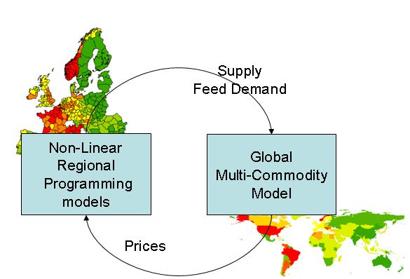
Figure 1: General structure of the CAPRI model
Source: Own illustration
The CAPRI modelling system itself consists of specific data bases, a methodology, its software implementation and the researchers involved in their development, maintenance and applications.
The data bases exploit wherever possible well-documented, official and harmonised data sources, especially data from EUROSTAT, FAOSTAT, OECD and extractions from the Farm Accounting Data Network (FADN)3) . Specific modules ensure that the data used in CAPRI are mutually compatible and complete in time and space. They cover about 65 agricultural primary and processed products for the EU (see the Annex), from farm type to global scale including input and output coefficients.
The economic model builds on a philosophy of model templates which are structurally identical so that instances for products and regions are generated by populating the template with specific parameter sets. This approach ensures comparability of results across products, activities and regions, allows for low cost system maintenance and enables its integration within a larger modelling network such as SEAMLESS or the DG Clima modelling suite. At the same time, the approach opens up the chance for complementary approaches at different levels, which may shed light on different aspects not covered by CAPRI or help to learn about possible aggregation errors in CAPRI.
CAPRI is designed for scenario analysis. It is a comparative static model, which technically means that the market equilibrium simulated for a given point in time does not involve lags or leads of endogenous variables. If several points in time are simulated, these simulatons may be perfomed therefore in any order or in parallel4). Comparative static results are best interpreted as the long run outcome of some scenario, after all adjustments to the new equilibrium are completed. By contrast, dynamic or recursive dynamic models also trace the adjustment path over time, while considering lagged relationships that are ususally critical in adjustment processes. CAPRI simulations start from a so-called baseline, which is a special applicaiton of the model as discussed in a separate chapter of this documention. The CAPRI baseline integrates projections from external sources, typically the Agricultural Outlook published annually by the European Commission's Directorate-General for Agriculture and Rural Development (DG-AGRI) (European Commission 2017). The parameters describing the reactions in the sector are calibrated to the baseline scenario, making the model behave in accordance with the data and projections. The baseline mirrors the projected agricultural situation up to some point in time and usually assumes status quo policy assumptions (currently: CAP 2014-2020). In a simulated scenario, all conditions in the baseline are maintained – except for the changes to be analysed.
CAPRI contains two modules, market and supply, which interact (see Figure 1).
The supply module consists of independent aggregate non linear programming models representing activities of all farmers at regional or farm type level captured by the Economic Accounts for Agriculture (EAA). The models optimize regional agricultural income, given the prices for inputs and outputs, subsidy levels and other policy measures. These models are a kind of hybrid approach, as they combine a Leontief-technology for variable costs covering a low and high yield variant5) with a non linear cost function which captures the effects of labour and capital on farmers’ decisions. The non linear cost function allows for perfect calibration of the models and a smooth simulation response rooted in observed behaviour (see also Jansson and Heckelei 2011).
Around 55 agricultural inputs produced in about 60 activities are covered in the supply module. The activities include inputs to crop and livestock production from other sectors and intermediate inputs produced by the farms such as feed and young animals. The models capture in high detail the premiums paid under CAP, include NPK balances and a module with feeding activities covering nutrient requirements of animals.
Main constraints outside the feed block are arable and grassland – which are treated as imperfect substitutes -, and potential policy restrictions (set-aside obligations, milk and sugar quotas, environmental constraints). Prices are exogenous in the supply module and provided by the market module. Grass, silage and manure are assumed to be non tradable and receive internal prices based on their substitution value and opportunity costs. A land supply curve renders agriculture responsive to returns to land. Non-agricultural areas respond in line with a given total region area, giving rise to land transitions.
Market equilibria are calculated by iterations between the supply module and the market module.
The market module for marketable agricultural outputs is a spatial, non-stochastic global multi-commodity model for about 65 primary and processed agricultural products. About 80 world regions are modelled, but aggregated to about 40 trade regions that trade bilaterally with each other, with the possibility of simultaneous import and export. It simulates supply, demand, and price changes in global markets considering international trade.
Agricultural supply is modelled in a simpler way than in the supply module, with behavioural functions for supply and feed demand. These are supplemented with other functions for processing, biofuel use, and human consumption. These functions apply flexible functional forms where calibration algorithms ensure full compliance with micro economic theory including curvature. The parameters are synthetic, i.e. to a large extent taken from the literature and other modelling systems.Consumers and traders are represented by economic agents that follow neo-classical micro-economic theory regarding behaviour, which makes it possible to compute welfare effects. Bi lateral trade flows and attached prices are modelled based on the Armington assumptions (Armington 1969). Policy instruments cover (bi lateral) tariffs, the Tariff Rate Quota (TRQ) mechanism and, for the EU, intervention stocks and subsidized exports. This market module delivers prices used in the supply module and allows for market analysis at global, EU and national scale.
As the supply models are solved independently at fixed prices, the link between the supply and market modules is based on an iterative procedure. After each iteration, during which the supply module works with fixed prices, the constant terms of the behavioural functions for supply and feed demand are calibrated to the results of the regional aggregate programming models aggregated to Member State level. Solving the market modules then delivers new prices. A weighted average of the prices from past iterations then defines the prices used in the next iteration of the supply module. Equally, in between iterations, CAP premiums are re calculated to ensure compliance with national ceilings and crop yields may respond to changing market prices.
Environmental indicators, primarily for nutrient surpluses and greenhouse gas (GHG) emissions, are calculated in CAPRI and may be directly addressed in some scenarios. Regarding nutrient surpluses, the supply module contains nutrient balance equations for nitrogen, phosphorous and potassium. It considers nutrient uptake by crops following a crop growth function, and supply of nutrients from mineral fertilizer, manure, crop residues, and, for nitrogen, atmospheric deposition and fixation. The balances also contain factors for over-fertilization, loss rates, and nutrient availability per source. From those balances nutrient surpluses can be calculated per region of the supply model. Technical information from the supply module is used to compute greenhouse gas emissions, based on IPCC methodology6). Globally, GHG emissions are computed based on estimated emission intensities per ton of product and production levels for globally traded commodities.
CAPRI allows for modular applications as e.g. regional supply models for a specific Member State may be run at fixed exogenous prices without any market module. In previous applications farm heterogeneity has been represented by a set of farm types for each NUTS2 region, each with its own supply model. The farm type model layer is currently being replaced with another solution such that it has been switched OFF in recent applications. Equally, the global market model can be run in stand-alone mode as well.
Post-model analysis includes the calculation of different income indicators as variable costs, revenues, gross margins, etc., both for individual production activities as for regions, according to the methodology of the EAA. A welfare analysis at Member State level, or globally, at country or country block level, covers agricultural profits, tariff revenues, outlays for domestic supports and the money metric measure to capture welfare effects on consumers. Outlays under the first pillar of the CAP are modelled in very high detail. Among the post model analysis options there are some designed to disentangle various contributions to scenario effects as explained in Chapter 6. An important element of post model analysis is the option of spatial down-scaling part to clusters of 1×1 km grid cells, covering crop shares, crop yields, animal stocking densities, fertilizer application rates and derived environmental indicators. This is based on a statistical approach, handeled in file capdis.gms and covered in a separate Chapter of this documentation. Model results are presented as interactive maps and as thematic interactive drill-down tables. The CAPRI graphical user interface including the exploitation tools are documented in a separate user manual7).
More information about the CAPRI model, including technical documentation, lists of peer-reviewed and other publications, and open access to the modelling system, is available at the model webpage: www.capri-model.org.