CAPRI Online Manual (update)

A key element in analysing policy changes from an economic viewpoint is to look at welfare changes. The “classical” elements of a welfare analysis are changes in consumer and producer rents and for the tax payer. That concept is also followed in CAPRI.

For consumers, CAPRI uses the money metric concept. It can be broadly understood as a measurement for changes in the purchasing power of the consumer. The concept is also linked to the expenditure function as introduced in Section 5.4.4 :

\begin{equation} M(cpri^r,cpri^s,Y^r )=e(cpri^r,U(cpri^s,Y^r )) \end{equation}

Where e(.) is the expenditure function, \(Y^r\) is expenditure in the reference situation, and \(cpri^r (cpri^s)\) is the price vector in the reference (scenario) situation. The money metric is thus the expenditure the consumer would need at reference prices to be as well of as if facing the scenario prices at reference income. The difference of money metric for a given scenario to money metric in the reference situation is the equivalent variation. Considering the generalised Leontief form of the indirect utility function used in CAPRI (compare with Section 5.4.4 ) we get

\begin{align} \begin{split} e (cpri^r, U(cpri^s,Y^r)) &= \left\{ F^r+ \frac{G^r}{G^s⁄(Y^r-F^s)}-Y^r \right\}+Y^r \\ & = \left\{ \frac {G^r}{G^s}(Y^r-F^s )-(Y^r-F^r ) \right\}+Y^r \end{split} \end{align}

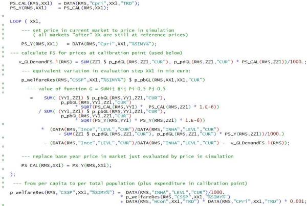
The bracket {} is the equivalent variation of the change from the reference to the scenario situation. In the code (in gams\reports\welfare.gms) the momey metric is computed in a loop over products such that the contributions of single products are displayed¹⁾. It is also considered that the per capita demand needs to be multiplied with population.

For some agents the welfare accounting involves particularities for those regions covered by the regional programming models that will be discussed below. In the general case (for “non supply model regions”) producer welfare may be derived in the market model from the normalised profit function underlying the supply functions and the input demands for feed energy and land:

\begin{equation} \pi(p^s)=π_0+\sum_x as_x p_x^s+0.5 \sum_{x,y} bs_{x,y} p_x^s p_y^s \end{equation}

where \(p^s\) is the price vector in the scenario situation and the arbitrary constant \(\pi_0\) has been chosen as 50% of reference run revenues. In order to show the changes in producer welfare by product we compute producer welfare in the scenario as follows: