This is an old revision of the document!
Table of Contents
The Complete and Consistent Data Base (COCO) for the national scale
The COCO database is built by the application of two modules:
COCO1 module:
Prepare national database for all EU27 Member States the Western Balkan Countries, Turkey and Norway.
It is basically divided into three main parts:
- A data import “part” that is not a single “module” but rather a collection activity to prepare a large set of very heterogeneous input files
- Including and combining these partly overlapping input data according to some hierarchical overlay criteria, and
- Calculating complete and consistent time series while remaining close to the raw data.
Data preparation (part 1) and overlay (part 2) form a bridge between raw data and their consolidation to impose completeness and consistency. The overlay part tries to tackle gaps in the data in a quite conventional way: If data in the first best source (say a particular Eurostat table from some domain) are unavailable, look for a second best source and fill the gaps using a conversion factor to take account of potential differences in definitions. To process the amount of data needed in a reasonable time this search to second, third or even fourth best solutions is handled as far as possible in a generic way in the GAMS code of COCO where it is checked whether certain data are given and reasonable. However there are a few special topics that are explained in separate sections.
COCO2:
The finishing step estimates consumer prices, consumption losses, and some supplementary data for the feed sector (by-products used as feedstuffs, animal requirements on the MS level, contents and yields of roughage). Both tasks run simultaneously for all countries and build on intermediate results from the main (COCO1) part of COCO like human consumption and processing quantities.
Overview and data requirements for the national scale
An overview on the key data collection, assingments and corrections in main program coco1.gms is given in the following figure.
Figure 2: Overview on key elements in the consolidation of European data at the Member state level (in coco1.gms)
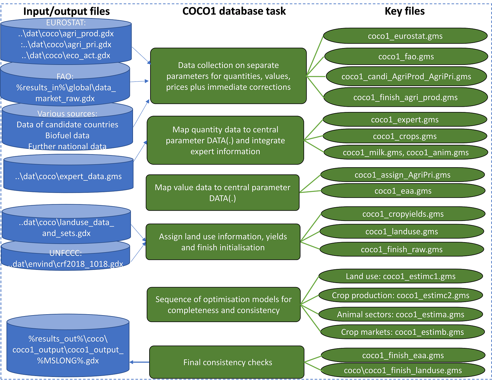
Source: Own illustration
The different steps will be explained in more detail in the following sections.
The CAPRI modelling system is, as far as possible, fed by statistical sources available at European level which are mostly centralised and regularly updated. Farm and market balances, economic indicators, acreages, herd sizes and national input output coefficients were initially almost entirely from EUROSTAT. In the course of time, more and more special data sets have been added to fill gaps or resolve problems detected in EUROSTAT data, such as specific data on Western Balkan Countries or on the biofuel sector.
The main sources used to build up the national data base are shown in the following.
Table 3: Data items and their main sources
| Data items | Source |
|---|---|
| Activity levels | Eurostat: Crop production statistics, Land use statistics, herd size statistics, slaughtering statistics, statistics on import and export of live animals For Western Balkan Countries and Turkey: Eurostat supplemented with national statistical yearbooks, data from national ministries, FAOstat production statistics and others |
| Production, farm and market balance positions | Eurostat: Farm and market balance statistics, crop production statistics, slaughtering statistics, statistics on import and export of live animals For Western Balkan Countries and Turkey: Eurostat supplemented with national statistical yearbooks, data from national ministries, FAOstat production statistics and others |
| Sectoral revenues, costs, and producer prices | Eurostat: Economic Accounts for Agriculture (EAA) and price indices for gap filling, otherwise unit value calculation For Western Balkan Countries and Turkey: Supplemented with national statistical yearbooks, data from national ministries, results from AgriPolicy, FAOstat price statistics |
| Consumer prices | Derived from macroeconomic expenditure data (Eurostat, supplemented with UNSTATS) and food price information from various sources |
| Output coefficients | Derived from production and activity levels, engineering knowledge |
Data Import
A large set of very heterogeneous input files (in terms of organisation and format) is collected, currently covering the following years:
Table 4: Temporal coverage of national data by region
| Member State | Range |
|---|---|
| EU15 Member States without Germany | 1984 – 2014 |
| Germany and (12) New Member States | 1989 – 2014 |
| Western Balkan (WB) Countries and Turkey | 1995 – 2014 |
| Norway | 1984 – 2014 |
Eurostat data
First step: Data download and format conversion Data are originally downloaded in “TSV-format”, as offered by Eurostat for bulk data users. The TSV-format is a flat file format for time series. Data can be selected for all EU MS and some Candidate Countries. Availability differs by country, of course (almost nothing for the Kosovo, Montenegro, Bosnia & Herzegonina). In the process of downloading the TSV files are also converted in GAMS readable form (csv or gdx). The following themes and table groups of Eurostat are accessed:
Agriculture, forestry and fisheries
- Agriculture (“agr”)
- Economic Accounts for Agriculture (Table Group “aact”, saved on CAPRI parameter “p_ecoact”
- Agricultural prices and price indices (Table Group “apri”, saved on CAPRI parameter “p_agripri”
- Agricultural product related physical information (production, activity levels from Table Group “apro”, saved on CAPRI parameter “p_agriprod”
- Older, discontinued Eurostat series that still provide useful information (requiring some ad hoc extrapolations), for example (a) market balance information for products other than cereals, oilseeds and wine, critical for “COCO1”, (b) relative price level indices of food products (MS relative to EU average) for COCO2, © availability and production of feedingsstuffs (useful for COCO2 completions on feed from by-products)
Economy and Finance
- National annual accounts (“nama10”)
- Annual national accounts → National Accounts detailed breakdowns (by industry, by product, by consumption purpose) → Final consumption expenditure of households by consumption purpose (COICOP 3 digit),
- General indicators to National Accounts - Population and employment
- GDP and main components - Current prices, volumes, price indices
- Prices (“prc”)
- Harmonized indices of consumer prices (prc_hicp) here: HICP (2005=100) -annual Data, and HICP - Item weights
Second step: data selection and code mapping The second step is data selection and code mapping performed by the GAMS program ‘coco_input.gms’. Cross sets linking Eurostat codes to COCO codes define the subset of data series subsequently used.
The mapping rules are collected in two sub-programs called by ‘coco_input.gms’, for example:
- ‘gams\coco\ eurostat_agriculture_mapping.gms’ for the tables from Eurostat’s “Agriculture and Fisheries” Statistics
- ‘eurostat_ econfinc_mapping.gms’ for the tables from Eurostat’s “Economy and Finance” Statistics
Example from file ‘Eurostat _agriculture_mapping.gms’
| SET AgriProdOriEurostat / apro_acs_a_C1000_AR “CEREALS-EXCLUDING RICE-AREA” apro_acs_a_C1110_AR “COMMON WHEAT AND SPELT - AREA” SET AgriProd_MAP(ASS_COLS,ASS_ROWS,AgriProdOriEurostat) / CERE.LEVL. apro_acs_a_C1000_AR SWHE.LEVL. apro_acs_a_C1110_AR |
The results of the program run are gdx-files loaded by files (e.g. coco\coco1_eurostat.gms) which are in turn loaded by coco1.gms or coco2.gms.
Western Balkan Countries and Turkey
For those countries Eurostat data need completion in almost every area which is handled in country specific xls files. The structure of these supplementary Excel country sheets and the definitions of the data are tailored to COCO. The resulting sheets in these xls files are uniform across countries, in order to ease data extraction for the modelling part by applying macros. However, each national information system has its own peculiarities and hence, not all data are fully harmonised across countries. Various sources are assessed and combined in a case by case manner: Eurostat data, if already available and plausible, are handled as the preferred data source. Data collected from the national statistical yearbooks have second priority, followed by expert data collected in from earlier projects. Finally FAO data provides often the fall-back solution for any remaining missing time series.
The final sheet in each of these country specific xls files is the interface to the GAMS programing world of COCO. An Excel macro “SELECT_data_all” collects the time-series compiled in other sheets and puts them into this final sheet with the appropriate COCO code. Another macro finally exports the numbers into text files like “dat\coco\bosnia_coco.gms”. Because the xls file are quite complex due to various linkages, we do not read directly from them. This avoids unplanned changes and permits convenient tracing of data changes via the CAPRI versioning system svn.
Supplementary data for Romania and Bulgaria
Country level data from national experts were compiled in Excel files that help in particular to complete the meat and milk sectors.
FAO data selection
Two FAO data sources are combined:
- For all regions FAO data (mapped in the context of module “global database” to CAPRI codes and hence consistent across modules) serve as a fall back option under certain conditions, defined in the code. This fall back function of FAO data has gained in importance since Eurostat discontinued the publication of most market balances since 2014. In some cases also activity level (area) information may be taken from FAO.
- Some particular data like disaggregate data on herds of chicken, ducks, turkeys and geese are compiled in a separate include file dat\coco\fao_add.gms because these data types are usually not loaded for global database.
Other additional input data
COCO1: Biofuels
- Production, market balance and feedstock quantities for biodiesel and bioethanol are collected from a multitude of sources:
- EU project www.elobio.eu (production, demand, biodiese and bioethanol, 1999-2007)
- Eurostat, Energy balances and demand (tables nrg_xxxx) production, demand, trade for diesel, gasoline, biodiesel and bioethanol, 2001-15)
- Eurostat, Production and trade (PRODCOM), ethanol and biodiesel, 2000-14
- PRIMES model1) database (production, biodiesel and bioethanol, 2000-07)
- US Energy Information Administration (EIA), production of biodiesel and bioethanol, 2000-12, incl. some non-EU countries
- DG Agri Ethanol balances (production partly with split by feedstocks and MS, demand and trade)
- Aglink ex post database (most data for Turkey, also EU biofuel production from non-standard sources (NAGR).
- USDA GAIN reports (market balances for Serbia, feedstocks for biodiesel in EU)
- FAOstat (market balances for palm oil)
- Prices at the pump and retail prices for diesel and gasoline are from Eurostat’s energy database (http://epp.eurostat.ec.europa.eu/portal/page/portal/energy/data/database), supplemented with IEA Statistics 2016 for Turkey.
- Taxes for diesel, gasoline, biodiesel and bioethanol are collected from DG Energy website and publications, and EURACTIV, EU news & policy debates, Brussels (http://www.euractiv.com/en/enterprise-jobs/fuel-taxation/article-117495)
- Some supplementary Aglink data give information on feedstock composition, tariffs and world market prices for crude oil, biodiesel and bioethanol.
- Trade data for undenatured ethyl alcohol, denatured ethyl alcohol, fatty acid mono-alkyl esters, crude palm oil, palm and fraction and palm kernel and fraction are collected from Eurostat’s COMEXT data (2000-14).
- Market balances for palm oil are taken from FAOstat and supplemented with COMEXT.
COCO1: Sugar Quotas
- All sugar quotas 1999 until 2006 from the annual sugar yearbook.
- Buy-back 2006 in the restructuring program from CAP monitor 16 January 2008.
- Sugar quotas renounced by member states following sugar reform (2006-2010), information from Wirtschaftliche Vereinigung Zucker e.V. (WVZ) and Verein der Zuckerindustrie e.V. (VdZ), Bonn (http://www.zuckerwirtschaft.de/1_3_2_1.htm) and KWS SAAT AG, Einbeck (http://www.kws.de/ca/fh/thd/)
COCO1: Milk
- Market balances for casein and whey powder were only available on EU level from ZMP, Bonn, which was closed down in 2009.
- DG Agri partly completes gaps in Eurostat series and offers this consolidated database for download. This is used to close gaps in gams\coco\coco1_eurostat.
COCO1: Producer prices for cotton
Import unit values for cotton seeds, cotton lint, flax and hemp are additionally selected from COMEXT.
COCO1: Expert data
Data from experts, which will overwrite all Eurostat data, is included for special issues for some Member States (e.g. grass yields for the Netherlands).
This also applies at the moment for all Norwegian input data such that Eurostat data are currently ignored. However, as Eurostat completeness has also improved on Norway, this procedure might be reconsidered in the future.
COCO1: Land use data
The raw data on land use are currently prepared outside the CAPRI system. Source code and input files are available at EuroCARE, Bonn (R:\Coco_input\land_use). Relevant (raw) information is stored in dat\coco\landuse_data_and_sets.gdx. The data base comprises information on land use classes from various sources, which are again partly discontinued but useful for the early years:
- REGIO - Eurostat, land use, REGIO domain( NUTS2 level - yearly, 1984-2014)
- ENVIO - Eurostat, land use, env_la_luc1.xls (MS level - 1985, 1990,1995, 2000)
- LANDCOVER - Eurostat, land cover(MS level – 2009, 2012, 2015)
- Corine Land Cover (CLC), 44clc_nuts2.xls (NUTS2 level - 1990, 2000, 2006, 2012)
- FAO - area.xls(MS level - yearly, 1984-2016)
- MCPFE (Ministerial Conference on the Protection of Forests in Europe), jointly published by FAO and UNECE (MS level - 1990, 2000, 2005, 2010, 2015)
- FSS - Eurostat, FSS(NUTS2 level - 1990, 1993, …, 2007, 2010, 2013), only added in coco1\landuse
- UNFCCC (1990-2016), also covers land transitions and settlement data. Official data for LULUCF accounting, merged with other data in coco1_landuse.
COCO2: Economic data
- Eurostat: Economy and Finance, Exchange rates, Bilateral exchange rates, Euro/ECU exchange rates. Data is already prepared in Excel for premature introduction of Euro in price data from the International Labour Organisation (ILO).
- Eurostat, population. To complete early years data from and old Eurostat domain (AGRIS, Population) are also loaded.
- GDP price index expressed in Euros
COCO2: Expenditures
Consumer expenditures on food items are included from:
- Eurostat: Old domain SEC2 for data up to 1997 (HIST)
- Instituto Nacional de Estadística m(INE): Anuario de Estadística Agroalimentaria (AEA), Consumer expenditure on food items in Spain close to HIST definitions up to 1996
- Rheinisch-Westfälisches Institut für Wirtschaftsforschung (RWI): Consumer expenditure on food items for DEW 1985-92 in Mio DM
- Statistisches Bundesamt Deutschland (SBA): Weighted average of expenditure shares in German household types 2 and 3 (1985-91)
- Eurostat, Final consumption expenditure of households by consumption purpose (COICOP 3 digit)
- United Nations Statistics Division (UNSTATS): Household consumption expenditure in USD
- Eurostat, PRICE: Consumer expenditure weights are used as indicators for budget shares
- Eurostat: Economy and Finance, GDP and main components, Final consumption expenditure of households: Total private consumption of households in current prices (Table “a_gdp_c”)
COCO2: Consumer food prices and consumer food price indices
Food price indices from:
- Eurostat, PRICE, 2005=100.
- Several national sources for western Balkan regions
- Eurostat: Old domain FOOD of section AGRICULTURE: Aggregate food price index with old Eurostat methodology and base 1985
- INTERNATIONAL LABOUR ORGANIZATION Geneva (ILO): LABORSTA Labour Statistics Database, retail prices of selected food unit, prices indices of selected food unit, discontinued after 2008
- Eurostat: Detailed average prices – 2008 - 2015 [table prc_dap15] is used to extend the ILO consumer price series.
COCO2: By-products
- FAO: Food Balance Sheets, Commodity Balances, Livestock and Fish Primary Equivalents: Imports and exports quantities for fish meal, dried cassava, gluten deed and meal, as well as feed quantities for fish meal.
- Eurostat: Purchase prices for fish meal, dried sugar beet pulp, soya cake, and wheat bran
- Eurostat: data (at most up to 2010) from discontinued tables (“food_in afeed1” and “bilares”) on production of feedingstuffs and availability of feedingstuffs
- FAO: Food Balance Sheets, Commodity Balances, Crop Primary Equivalents: Milled rice and total sugar unit value
- Netherlands Economic Institute (NEI): Purchase prices for sugar, calculated by the average of Intervention Price and CAOBISCO price
COCO2: Milk Products
- Zentrale Markt- und Preisberichtstelle (ZMP): Producer prices of selected milk products (only available for some countries)
- Agrarmarkt Informations-Gesellschaft mbH (AMI): AMI-Marktbilanz Milch 2011 (only available for some countries)
- DG AGRI (Réponses au questionnaire (art. 8 du Règlement (CEE) n° 536/93), (art. 15 R 1392/2001) and (art. 26 R 595/2004)): Data on direct sales of raw milk and farm processing in DG AGRI definitions for quota administration
COCO2: Others
- Eurostat: External trade, External trade detailed data, COMEXT, EU27 Trade Since 1988 By CN8, Reporter EU15: Auxiliary trade data for wheat, soft wheat and durum wheat, export values and quantities for cotton and cotton seeds, data on imports and exports of most relevant by-products
- Statistisches Jahrbuch ueber Ern., Landw. U. Forsten, 1999, 2006 und 2010 (Aufkommen u Verbrauch von Futtermitteln): Net imports and feed from domestic production of by-products in Germany
- USDA: Prices for soya, rape and sunflower cake and oil, prices for corn gluten feed
COCO1: Overlay from various sources
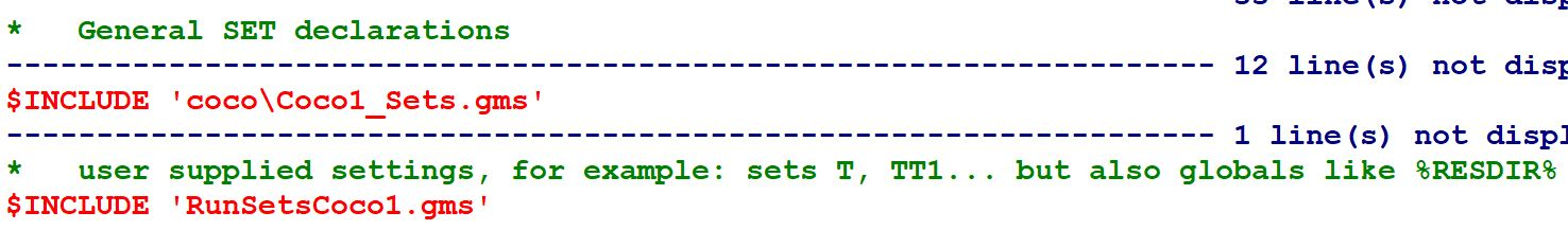
The main program coco1.gms starts with a number of declarations of sets and parameters to handle the collection and overlay of “raw data”, often given in a classification different from the target one (sets COLS, ROWS).
 A recurrent characteristic of COCO is to solve the problem: if the first best source has gaps in a particular country, or even is entirely empty, select the second or even third best source to fill the gaps.
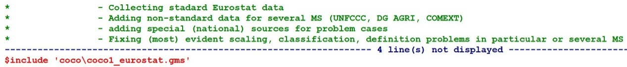
Including standard and supplementary data from Eurostat (‘coco1_eurostat.gms’)
The main program coco1.gms proceeds by importing data from Eurostat prepared beforehand (in coco_input.gms). The main data (on p_agriProd, p_ecoAct, and p_agriPri) are processed step by step and corrections made on selected data for all MS2).
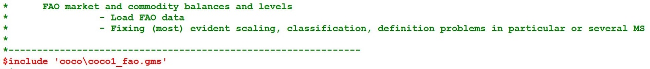
Data from FAOstat (‘coco1_fao.gms’)
The general fall-back option for missing data is FAOstat which requires a few corrections compared to the standard mappings in the context of module “global database”, including:
- Rebooking of “other use” to processing (PRCM) or other balance positions
- Disaggregation of olives (table olives, olives for oil), grapes (table grapes, grapes for wine), wheat (common, durum)
- Checks for data changes after sugar reform 2006
- Country specific fixes like in coco1_eurostat.gms.
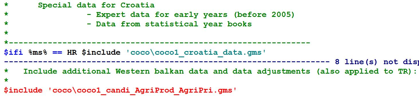
Data from additional sources for the Western Balkan Countries and Turkey (‘coco1_croatia_data.gms’ and ‘coco1_candi_AgriProd_AgriPri.gms’)
Croatia is the first country singled out from the special data input for the Western Balkan Countries and Turkey. Croatia is by now mostly sourced from Eurostat, as the other EU members, but a few supplementary expert data have been retained. For the other Western Balkan regions and Turkey, ‘coco1_candi_AgriProd_AgriPri.gms' further adapts the WB data from the country specific xls files to match the COCO definitions that also apply to EU28 countries (on parameters p_agriProd and p_agriPri).
The include file handles the following:
- Similar to EU-28 MS there are many case-by-case adjustments correcting different scaling and definitions (live weight ↔ carcass weight, reaggregations for wine and fruits…).
- In many cases, market balances are simply incomplete. As a fall back solution, domestic demand is calculated from production and net trade and disaggregated with shares taken from a sister country aggregate (Romania, Bulgaria, Greece, Slovenia, Hungary). Other corrections with “borrowed” information are:
- Trade data are frequently missing in the WBs, such that FAO data are included where available.
- Production of oilcakes and sugar is estimated from raw products, if missing, using the sister country aggregate processing coefficients;
- The production of milk products is estimated from processing coefficients in Serbia which has a quite complete series;
- Price information is also completed relying on the sister country aggregates.
Final completions and revisions for all Member States (‘coco1_finish_agriprod.gms’)
Based on the availability of second and third best options various finalising steps are applied to the quantity data. It should be noted that the CAPRI database tries to estimate market balances (needed for separate behavioural function for feed, food, processing, biofuel demand) in spite of Eurostat discontinuing the publication of market balances for most products since 2014. For this purpose the old Eurostat market balances are still loaded and combined with more recent production data. This triggers the need for data completions and estimations in the most recent years (which are also most critical for projections). In 2019 market balance data have returned to the Eurostat server for cereals and oilseeds, but only for a single year (2017) ⇒ It is likely that adjustments like the following will also be needed in the future:
- Completion of production data from the (discontinued) Eurostat market balance statistics (model code “USAP”) with quantity information given from the production statistics (code “GROF”) or from agricultural account statistics (model code “EAAQ”) using a correction factor calculated from overlapping years.
- Additional gap filling using FAO data for special cases and general cases of missing data (e.g. for balances). An additional difficulty is that FAO commoditiy balances are currently (2019) also ending in 2013 (especially valuable for recent years).
- Domestic use can be calculated (under some conditions) from imports, export and usable production. If only domestic use is given for some products, the sub-positions, such as industrial use, processing, human consumption, feed on market, total seed and total losses are allocated with the average shares in data for other years, from the same country. As a fall back solution, the average shares from other countries are used.
- For the milk products whey powder and casein, the disaggregation of demand is mainly based on EU data collected by the German “Zentrale Markt- und Preisberichtstelle für Erzeugnisse der Land-, Forst- und Ernährungswirtschaft GmbH” (ZMP) and some auxiliary assumptions.
- As data for oilseeds are critical for all countries, the implied processing coefficient is checked for plausibility. If the national coefficient is lower than 60% or above 150% the average coefficient for all EU-15 MS, the data for usable production of the country are corrected by multiplying the processing data with the average EU-15 coefficient. Domestic use and all sub-positions are subsequently re-calculated.
- Some additional calculations to prepare the use of animal herd data in coco1_anim:
- Some calculations to combine FAO and FSS data on poultry herds
- Completions acknowledging seasonality in cattle and sheep and goats herd countings
- Aggregations and residual calculations to the COCO animal categories from animal types in Eurostat (say “Heifers for raising, 1-2 years”)
The file handling the previous actions is ‘coco1_finish_agriprod.gms’:

The previous code snippet also shows for the interested reader two frequently used debugging devices:
- The key parameters at a certain point in the program flow (above: p_agriProd, p_agriPri, p_ecoAct) are copied to a debugging parameter “debug” (better name would be: “p_debug”). At the end of a coco1 run (or if desired also at this point) the parameter is unloaded into a file “results\coco\debug\debug_%MS%.gdx” such that the various assignments, corrections, deletions that have occurred up to a certain program line may be inspected in one file.
- The next command “$batinclude “util\debug” %system.fn% %system.incline% unloads the whole memory, incuding all parameters but also sets and other symbols, at this point into a debugging file in the gams\temp folder. This may be useful to analyse “difficult” cases of debugging.
Finally the biofuel sector is prepared.
EU biofuel sector data (‘coco1_finish_agriprod.gms’ and ‘prepare_biofuel_data.gms’)
The first issue to note is that market balances for sugar beet and sugar are compiled in such a way that all biofuel use of beets is converted into biofuel use of sugar, as if the beets were first processed to sugar and only then converted to ethanol. The advantage of this approach is that sugar is part of the market model and thus may enter the behavioural functions for biofuel feedstock use whereas beets only exist in the supply part of CAPRI. A second advantage is that biofuel feedstock use was indeed booked under sugar in some MS and under beets in others such that our approach ensures a standardisation of booking principles.
Biofuel production
There is no differentiation made between fuel- or non-fuel (undenatured or denatured) quantities in production, import and export positions of ethanol. But the consumption position of ethanol is differentiated in fuel-ethanol consumption and non-fuel-ethanol consumption. Hence data on fuel and non-fuel production and consumption of ethanol was required. In the case of biodiesel this differentiation is irrelevant. The ex-post data on biofuel production are coming from diverse sources which is unavoidable to complete the data for years as of 2002 up to the present, if necessary with the help of second and third best solutions or assumptions (compare biofuel\prepare_biofuel_data.gms).
The overlay considers data availability and consistency across sources:
- For ethanol we consider DG agri as the first best source as it does not only cover production and demand, but also a break down by feedstocks (cereals, beets, wine, fruits, potatoes, other).
- Some countries (Croatia, Turkey, Bulgaria, Romania, Serbia) are supplemented from other sources (AGLINK-COSIMO, USDA, Eurostat PRODCOM). AGLINK also supplements production other than from agricultural feedstocks.
- Eurostat PRODCOM, Energy balances and PRIMES serve to extrapolate or backcast the DG Agri information to years with missing data.
- Ethanol trade by MS is taken from COMEXT but scaled to be in line with DG AGri data for the whole EU.
- Production of biodiesel is usually from the energy balances while trade is from COMEXT. If data are complete and results reliable, demand is computed residually. In cases of missing data or implausible results, demand is taken from Energy balances, PRIMES, or the EloBio project and trade is calculated as a residual with some rules.
Feedstock demand
In addition to market balances for the fuels the CAPRI data base requires the shares of the raw products on the production of biodiesel and bioethanol at the level of CAPRI products. For bioethanol, this information is partly provided by the DG Agri balances, hence this has been selected to be the major source. The detailed recording follows from the existence of support measures for distillation of wine, fruits and potatoes which triggered a detailed monitoring of ethanol markets. However, for biodiesel the statistical sources are scarce. It turns out that the most consistent estimates for EU regions are apparently produced by USDA services, covering rape, sunflower, soya, palm oil but also used cooking oils, tallow and other oils. As these data do not cover single MS an estimation procedure has been devised (in biofuel\calc_feedstock_shares.gms). The initialisation of this estimated feedstock composition relied on the observed increase in INDM according to Eurostat (or more precisely the COCO initialisation when entering ‘prepare_biofuel_data.gms’) which is assumed to be the main source to “cut out” the required biofuel processing quantities (BIOF) by MS from market balances that so far did not include BIOF.
A special case was palm oil, as the CAPRI database (COCO) doesn’t cover an industrial use position for this product so far. EUROSTAT-COMEXT delivers data on import and export quantities of crude palm oil (HS 151110) for EU Member states. Thereby an increase of palm oil imports was observed within the relevant ex post period (2002-2005). Thus the following assumptions were made to derive approximated values for palm oil processing to biodiesel: (a) Import quantities minus export quantities are equal to domestic consumption of palm oil as domestic production in European Member states can be neglected. (b) The average aggregated consumption quantity of palm oil before 2002 was assumed to be completely used for human consumption as no significant biodiesel consumption took place. By subtracting this constant share of human consumption from the observed consumption quantities after 2002 gave an estimate for the quantities used for industrial processing
Given that many data sources are combined and several aggregation conditions should be maintained, it turned out necessary to set up a small optimisation problem with the following properties (see towards the end of ‘prepare_biofuel_data.gms’):
- The estimation tries to stay close to the initial feedstock composition
- Extra terms penalise deviations from DG Agri (first best souce for ethanol) and implausibly high shares for palm oil
- Technical conversion coefficients (see below) link standard feedstock use and estimated production which has to aggregate with non-standard feedstocks (NAGR) to total production of biofuels. Non-standard feedstocks are those not endogenous in the CAPRI market model (potatoes, fruits and other for bioethanol, used cooking oils, tallow and other for biodiesel)
- Total domestic use (with data modifications heavily penalised in the objective) is consistently broken down into biofuel use, other industrial use and non-industrial (e.g. food) use to avoid disturbing the initialisation in previous include files based on Eurostat data.
Technology parameters
Conversion coefficients for 1st generation biofuels were collected from different sources. The AgLink-Cosimo model includes a set of conversion coefficients which are in line with the CAPRI product definitions and have become the main source for CAPRI. The table below displays the set of conversion coefficients used for 1st generation biofuels and corresponding by-products.
Table 5:Conversion coefficients for 1st generation biofuel production
COCO1 Estimation procedure
COCO was primarily designed to fill gaps or to correct inconsistencies found in statistical data and, additionally, to easily integrate data from non EUROSTAT sources in the model. However, given the task of having to construct consistent time series on yields, market balances, EAA positions and prices for all EU Member States, and therefore thousands of series, a heavy weight was put on a transparent and uniform econometric solution so that manual corrections were avoided, to some extent at least. Regarding the construction of the data base, three principal problems had to be solved:
- Gaps had to be filled in time series, either before the first available point, inside the range where observations are given, or beyond it.
- Some time series were missing altogether and had to be estimated, e.g. when there are data on animal production but none on meat output per head.
- Corrections of given statistical data should be minimised, if possible.
In order to take into account logical relation between the time series to fill, and eventually to make minimal corrections in the light of consistency definitions, simultaneous estimation techniques are used in this exercise. In order to use to the greatest extent the information contained in the existing data, the following principles are applied:
- Accounting identities positions of the market balance summing up to zero, the difference between stocks as the stock change and similar restrictions constrain the estimation outcome.
- Relations between aggregated time series (e.g. total cereal area) and single time series are used as additional restrictions in the estimation process.
- Bounds for the estimated values based on engineering knowledge or derived from first and second moments of times series ensure plausible estimates and/or bind estimates to original data. Additionally, bounds are constructed from more disaggregated time series, if the aggregate is missing.
- As many time series as technically possible are estimated simultaneously to use the full extent of the informational content of the data constraints (1) and (2).
The first three points neatly conform to the Bayesian Highest Posterior Density (HPD) approach proposed in Heckelei et al. 2005. The reader may notice that the problem is quite similar to system estimation in economics. Consider a system of supply curves. A standard approach to estimate such a system includes the specification of a functional form consistent with profit maximisation and the imposition of various constraints (homogeneity, symmetry, convexity) on the parameters to be estimated. Our approach is quite similar, as our goal asks for consistent estimates as well. Instead, we introduce explicit data constraints involving the fitted values for each point and take the fitted values later as the content of the data base.
The estimation is prepared in the following steps:
- Estimate independent trend lines for the time series.
- Estimate a Hodrick-Prescott filter using given data where available and otherwise the trend estimate as input.
- Define ‘target values’ which are (a) given data, (b) the results from the Hodrick-Prescott filter times R² plus the last (1-R²) times the average of nearest observations. The target values may be considered modes of a prior distribution.
- Specify a ‘standard deviation’ for each data point which is different for given data and gaps.
The concept is put to work by a minimisation of normalised least squares under constraints:
\begin{align} \begin{split} min_{y_{i,t}} &\sum_{i,t\in obs} wgt^{dat}((y_{i,t}-y_{i,t}^{dat})/abs(y_{i,t}^{trd}-y_{i,t}^{dat}))^2\\ & + \sum_{i,t\notin obs} wgt^{ini}((y_{i,t}-y_{i,t}^{ini})/s_{i,t})^2\\ & + \sum_{i,t} wgt^{hp}((y_{i,t+1}-y_{i,t})-(y_{i,t}-y_{i,t-1})/s_{i,t})^2\\ & + \sum_{i,t} wgt^{up}((max(y_{i,t}^{up},y_{i,t})-y_{i,t}^{up}))/abs(y_{i,t}^{up}))^2\\ & + \sum_{i,t} wgt^{lo}((min(y_{i,t}^{lo},y_{i,t})-y_{i,t}^{lo}))/abs(y_{i,t}^{lo}))^2\\ \end{split} \end{align}
\begin{align*} \begin{split} &\text {s.t.}\\ &y_{i,t}^{LO}<y_{i,t}<y_{i,t}^{UP}\\ &\text {Accounting identities defined on} y_{i,t}\\ &\text {Identity of land use from different sources} \end{split} \end{align*}
where i represents the index of the elements to estimate (crop production activities or groups, herd sizes etc.), t stands for the year, wgtx are weights attached to the different parts of the objective (\(wgt^{dat} = wgt^{hp} = 10, wgt^{ini} = 1, wgt^{up} = wgt^{lo} = 100)\), and
\(y_{i,t}\) = the fitted value for item i, year t
\(y_{i,t}^{dat}\) = the observed data for item i, year t
\(obs\) = {\((i,t) | y_{i,t}^{dat} ≠ 0\)}, the set of data points with nonzero data
\(y_{i,t}^{trd}\) = the trend value of an initial t rend line through the given data
\(y_{i,t}^{ini}\) = initial supports for gaps: preliminary Hodrick-Prescott filter result (from step 2) times R² plus the last (1-R²) times the average of nearest observations
\(s_{i,t}, (i,t)\notin obs\) = \(0.1 \cdot y_{i,t}^{ini} +s_{i,t}^{trd}\) , weighted sum of the initial support for gaps and the standard error of the initialising trend
\(s_{i,t}, (i,t)\in obs\) = \(0.1 \cdot y_{i,t}^{dat} +s_{i,t}^{trd}\) , weighted sum of given data and the standard error of the initialising trend
\(y_{i,t}^{lo},y_{i,t}^{up}\) = ‘soft’ bounds, triggering a high additional penalty if violated
\(y_{i,t}^{LO},y_{i,t}^{UP}\) = ‘hard’ bounds, defining the feasible space
The general weighing of the different terms evidently reflects the acceptability of certain types of deviations which is lowest ( = 1) for deviations of the fitted value from the HP filter initialisation as these are considered quite poor, preliminary estimates (derived from independent trends). The weights are 10 times higher for deviations from given data and for the smoothing HP filter term. Finally there are extra penalty terms for fitted values moving beyond plausible ‘soft’ bounds \(y_{i,t}^{lo},y_{i,t}^{up}\). The ‘hard’ bounds \(y_{i,t}^{LO},y_{i,t}^{UP}\) are constraining the feasible space for a number of solution attempts. However, if it turns out that certain constraints would persistently preclude feasibility of the data consolidation problem, they are relaxed in a stepwise fashion, but this widening of bounds is monitored on a parameter to check.
The denominators used to normalise the different terms are ‘standard deviations’ of the prior distribution in the framework of a HPD estimation but they are specified in view of practical considerations. Essentially they provide another weighting for particular (i,t) deviations depending on their acceptability, but these weights are specific to the particular data point. All denominators are derived from the variable in question such that they acknowledge the fact that the means of the time series entering the estimation deviate considerably. The normalisation hence leads to minimisation of relative deviations instead of absolute ones which could not be summed in a reasonable way.
It should be mentioned that the above representation of the COCO objective function is a quite simplified one: It is evident that the above lacks safeguards against division by zero or very small values which are included in the GAMS code. Furthermore there are different types of gaps which are not reflected above to avoid clutter (Are there gaps in a series with some data or is the series empty? Is the mean based on data or estimated from \(y_{i,t}^{lo},y_{i,t}^{up}\) ?)
Equation 4 indicates that accountancy restrictions are added. These restrictions can be balances (land, milk contents, young animals), aggregation conditions, definitions for processing coefficients and yields etc. They are quite similar to those applied for the ex ante trend projections as discussed in detail in Section 3.3 but the COCO1 accounting identities tend to acknowledge more details or have to establish the data base that is subsequently given for the ex ante trend projections, for example related to the split of high and low yield animal activites (DCOL, DCOH, BULL, BULH, HEIL, HEIH):

The fixed yield variation imposed in this way is ± 20% and each of the variants corresponds a fixed 50% of the total activity level whereas other accounting equations ensure that the process length DAYS and the daily growth DAILY vary accordingly.
In the dairy sector the strategy of an update in 2015 has been to obtain a fairly detailed data consolidation with a distinction of milk processed and dairy products obtained in dairies and on farm, using most of the available data sources. For the subsequent modules this disaggregate description of the dairy sector is consolidated to some extent for further use.
The equation system considers that both in dairy as well as on farm the raw milk used has to be consistent in terms of milk fat and protein with the products obtained:
\begin{equation} PCRM_M \cdot \delta_{c,M}= \sum_i (NAGR_i- PRCM_i)\cdot \delta_{c,i} \end{equation}
where
\(PRCM\) = processing of raw milk M or dairy product i (e.g. cheese)
\(NAGR\) = products obtained in dairies (e.g. MC100, fresh products, from apro_mk_pobta)
\(c\) = type of milk content (= FATS, PROT)
\(i\) = dairy product (e.g. MC100, fresh products, from apro_mk_pobta)
\(\delta\) = average content in dairies
In a similar manner we have balances for milk contents in on farm use of raw milk as well as in the products obtained on farm:
\begin{equation} (INDM_M+HCOM_M)\cdot \delta_{c,M}= \sum_i FARM_i \cdot \phi_{c,i} \end{equation}
where
\(INDM\) = use of raw milk M on farm for farm cheese, farm butter etc (e.g. MF240-UWM)
\(HCOM\) = use of raw milk M on farm as drinking milk (MF110-UWM, includes both direct sales as well as home consumption)
\(FARM\) = products obtained on farm (e.g. MF110-PRO, MF240-PRO)
\(\phi\) = average content on farm
The content of milk products will typically differ, in particular for the most important product “fresh milk products” (FRMI), as this includes yoghurts etc in dairies but will be dominated by drinking milk on farm. However, to accomodate the important case of drinking milk it is not necessary to have all contents on farm deviating freely from the standard contents in dairies. Instead we require that
\begin{equation} CORF_{c,i}\cdot \delta_{c,i}=\phi_{c,i} \end{equation}
where
\(CORF\) = ratio of on farm content to the standard content
and CORF is contrained to equal to one except that we permit CORF $\neq$ 1 for FRMI.
Production in dairies and on farm may be added to obtain the total production that enters the market balances:
\begin{equation} MAPR_i=NAGR_i+FARM_i \end{equation} \begin{equation} MAPR_i=HCOM_i+PCRM_i+FEDM_i+NTRD_i \end{equation}
where
\(MAPR\) = Marketable production according to the (discontinued) Eurostat market balances (USAP-FRMI from apro_mk_bal_B4410_12)
or in terms of the commercially marketed quantities only:
\begin{equation} NAGR_i=(HCOM_i-FARM_i)+PCRM_i+FEDM_i+NTRD_i \end{equation}
The market balance for the raw milk looks as follows:
\begin{equation} GROF_M=PRCM_M+HCOM_M+INDM_M+FEDM_M+LOSM_M \end{equation}
where
\(FEDM\) = Feed use of raw milk (apro_mk_farm_MF520_UWM)
\(LOSM\) = Losses of raw milk (apro_mk_farm_MF600_UWM)
After solving the data consolidation according to the above equations the following rebookings will be useful for subsequent modules:
\begin{equation} MAPR_i'=NAGR_i \end{equation}
\begin{equation} HCOM_i'=HCOM_i-FARM_i \end{equation}
\begin{equation} HCOM_M'+FEDM_M'+LOSF_M'=HCOM_M-FDEM_M+LOSM_M+INDM_M \end{equation}
The first two of the previous equations transform the standard (total) market balances including on farm use and production into “commercial” market balances only which is useful for comparisons with some datasets. The last equation is active for a while already in COCO. It identifies \(HCOM_M'\) = raw milk for direct sales (regardless of in terms of drinking milk or on farm products), feed milk and \(LOSF_M'\) , an aggregate of losses and on farm use of milk by farm households themselves. The original position \(INDM_M\) is basically allocated to a part consumed on farm and that part of direct sales which occurs in processed form (farm cheese, butter…). As the form of on farm consumption is not modelled in CAPRI, items FARM, NAGR, INDM are not passed on to subsequent modules, only LOSF is passed on, because this needs to be accounted for when calculating deliveries to dairies (\(PRCM_M\)).
Related to land use data there are also a number of particularities and details. We have various sources reporting data on the same item (LEVL) that evidently contradict each other before the data consolidatuion. During the consolidation the following equation ensures the identity of land use areas among different sources (LEVCLC, LEVFAO etc):

Based on the previous constraint all other land related accounting restrictions only have to be checked for the item “LEVL”, while the objective functions minimizes deviation from supports of all sources. Accounting restrictions ensure consistency of crop activities with land use classes and their aggregates.
Complications in the consolidation of land use data are related to the use of UNFCCC data for 6 land use classes (set “LUclass”: CROP, FORE, ARTIF, GRSLND, WETLND, RESLND), because three of the UNFCCC land use classes (GRSLND, WETLND, RESLND) differ conceptually from “related” categories from other data sets. Thus it is only possible to specify some inequnalities and an aggregation condition as constriants:

The last equation illustrates that the land use accounting based on UNFCCC data (introduced in 2015) also involves the land use changes (LUCpos) into the 6 LU classes (and a corresponding condition for changes from those LU classes).
It should also be explained that Equation 1 is not applied simultaneously to the whole dataset because the optimisation would take too long. Instead it is applied to subsets of closely related variables:
- Land use and land balance (Estimation step 1 for preliminary LU results).
- Crop production (land balance + yields) for all crops simultaneously (Estimation step 2).
- Production, yields, EAA, market balances for groups of animals like “cattle” (Estimation step 3).
- Crop EAA + market balances for groups of crops, taking production from (2.) as given (Estimation step 4).
- As the crop level estimation or the other crop completions may have slightly changed aggregate areas, the land use estimation has to be repeated (Estimation step 5).
This procedure has developed as a path dependent compromise between computation time and presumed quality. It starts with an estimation of land use in combination with agricultural land balance, including the land transition between LU classes. This determines the utilisable agricultural area (UAA) and non-agricultural land use. Step 2 distributes crop areas within the fixed UAA from step 1 and estimates crop production and yields. Step 3 only tackles the complete animal sector data (activities, markets, EAA). The crop production is taken as given, when market balance and EAA are estimated for the crops and derived processed products (step 4). However, with all steps completed some final checks may modify the results (e.g. delete tiny activity levels or estimate another crop area from another crop output value and thus change the UAAR). Furthermore the crop estimation may have slightly changed the ratio of cropland to productive grassland. Therefore the accounting identities ensured in steps 1 are not necessarily fulfilled in a strict sence anymore. Hence a final reconciliation of land use is added for full consistency:
Figure 3: Overview on main estimations in for the consolidation of national data in Europe (in coco1.gms)

Results are not always fully satisfactory (perhaps impossible given some raw data). For example the resulting prices (unit values) are far from a priori expectations for a number of series, in particular less important ones. This is because, apart from some additional security checks, unit values are by and large considered a free balancing variable calculated to preserve the identity between largely fixed EAA values and fixed production (in coco1_estimb). The priority for EAA values has been reduced somewhat in recent years but a more thorough revision would require to estimate production, market balances and EAA simultaneously rather than consecutively (first $(a)$, then $(c)$ for crops). As this is infeasible for all crops at the same time the whole estimation would need to be split up differently in the crop sector, perhaps first for the aggregates and then within those.
Furthermore it should be mentioned that the main parts of COCO are handled in a program (‘coco1.gms’) looping over MS because there are no direct linkages between them. However, for practical reasons it will be useful to run COCO in country groups that have the same coverage of years. The longest series (as off 1984) can be established for EU153) countries except Germany. For the New MS it turned out that data before 1989 are often very unreliable and create considerable burden in the data maintenance. These countries (and Germany) are only completed for years from 1989 onwards therefore. Norway also offers reliable series as of 1984. In the case of the Western Balkan countries it is rather hopeless to provide very recent data as key data are still missing such that the series can only be completed from 1995 onwards. Furthermore for the Western Balkan counties it was necessary to transfer certain coefficients and shares from (previously consolidated) neighbouring countries to the Western Balkan, such that a certain sequence is necessary for a reasonable application of COCO1:
- Run COCO1 for EU28 countriesand Norway, either in one batch from the GUI or one by one (always with sub-steps 1 to 5).
- Run COCO1 for the set of candidate countries (Western Balkan and Turkey) on the reduced time span with given data (1995 – 2009). Because these use some shares and ratios from an average of selected EU28 countries the latter have to be consolidated first.
COCO2: Data Preparation
The data consolidation in COCO2 only covers a few special topics:
- producer prices of dairy products and vegetable oils
- consumer prices
- consumer losses and nutrient intake after losses
- feed stuff quantities without market balances (by-product, fish emal)
- loss rates of fodder for preliminary balancing of animal nutrients
- corrections of certain LULUCF coefficients based on UNFCCC
An overview is given in the following figure.
Figure 4: Overview on main elements in the finalisation step for the consolidation of national data in Europe (in coco2.gms)

In spite of only limited subtasks tackled in coco2.gms, the multitude of different data inputs is comparable to that in COCO1.
Include file ‘coco2_collect.gms’
Various input files are collected with some adjustments to match to CAPRI definitions and with some gap filling. As the consumer prices follow from a top down expenditure allocation problem, the input data range from macroeconomic information to very detailed prices of food items.
- Consolidated data from COCO1
- Macroeconomic information from Eurostat and UNSTATS: Exchange rates, population, GDP deflator, private consumption of households in current prices.
- Price index information: Aggregate food price index, relative (to EU) food price index, harmonised indices of consumer prices (HICPs) with item weights all from Eurostat
- Expenditure by product groups (from Eurostat and national sources)
- Auxiliary data for special cases (Prices for some milk products in selected countries, fish meal information etc)
- Country Sheets of the Western Balkan and Turkey: Exchange rate, inhabitants, inflation rate, food expenditure shares
- Disaggregate absolute consumer prices for selected narrowly defined food items (ILO and Eurostat)
Where available, producer prices for milk products were already included from Eurostat statistics (Agricultural prices and price indices) in COCO1. Completeness was not achieved in COCO1, however, because processed dairy products are not part of the EAA. Here we complete some gaps using price information for some Member States and (partly assumed) relationships among dairy product prices and their fat and protein contents. Data on total consumer expenditures as well as expentitures by food groups are included from various sources as described in Chapter 2.2.2.5, partly extended using general price index information.
Consumer price index weights and price indices for food aggregates (2005=100) are coming from Eurostat tables on HICP. Supplementary information for Albania, Bosnia and Croatia comes from national agencies. The price index weights are used to extend older series on food expenditure by product groups (say “meat”) which have been discontinued (see below under file coco2_shares.gms).
Finally we use very narrowly defined absolute consumer prices (e.g. for spaghetti) and price indices. The earlier years (before 2008) had been provided by ILO which has discontinued this activity. For a subset of those Eurostat offers matching information as “detailed average prices (table prc_dapYY) that has been used to extend the ILO series. These prices are mapped to CAPRI regions, products and units (‘coco2_ilo_addup.gms’).
Price indices for food and non-alcoholic beverages from HICP as well as the general food price index are used to complete the disaggregate ILO prices for single typical food items. (like “Wheat bread white unsliced not wrapped”) using a Hodrick-Prescott filter and the expectation that their changes should follow the price index informaiton collected.
Finally another HPD estimator is used to adjust the dissagregate prices to be (somewhat) in line with Eurostat information on relative food price levels across Europe.
Include file ‘coco2_shares.gms’
Expenditure shares are defined and completed top-down using simple OLS estimates against related statistical expenditure information or, as a last fall back option, based on a trend.
The food expenditure share completions start with data from COICOP level 3 giving results on food and non-alcoholic beverages. Further disaggregation relies on historical Eurostat data (HIST), on the above mentioned index weights from HICP and partly national data (Germany and Spain).
A conveninent expenditure group is potatoes as these expenditure shares may be extrapolated based on COCO1 human consumption multiplied by producer price as regressors for OLS.
COCO2: Estimation procedure
Include file ‘coco2_def.gms’
The approach to determine consumer prices is to distribute food expenditure on groups with consumption quantities given from COCO1 results such that endogenous consumer prices link endogenous expenditure with exogenous quantities. Deviations of estimated expenditure and consumer prices from their supports is penalised in an entropy framework. Estimation is done year by year, starting with the most recent year where hard data are usually available to a greater extent than for the oldest years in the database. Including consumer price changes (always relative to the previously solved year) serves to stabilise the results to some extent such that the objective does not only have supports for the consumer prices, but also for their changes. The entropy problem is solved by maximizing:
\begin{align} \begin{split} max_t &- \sum_{m,j,k} CPS_{m,j,2}*HCOM_{m,j,k}/1000/TOFO_{m,t}*\\ &PE_{m,j,k}*LOG(PE_{m,j,k}/PQ_k)\\ &-\sum_{m,j,k} CPS_{m,j,2}*HCOM_{m,j,k}/1000/TOFO_{m,t}*\\ &PED_{m,j,k}*LOG(PED_{m,j,k}/PQ_k)\\ &-\sum_{m,FOPOS,k} EXS_{m,FOPOS,2}/TOFO_{m,t}*\\ &PEX_{m,FOPOS,k}*LOG(PEX_{m,FOPOS,k}/PQ_k)\\ &-\sum_{m,j,k} PFAC_{m,k}*LOG(PFAC_{m,,k}/PQ_k)*1000\\ \end{split} \end{align}
where m represents the region, j the food item with consumer price, FOPOS the food group, t stands for the current estimation year, t_1 for the year estimated before and k for the number of support points (=3).
Parameters are
| \(HCOM_{m,j,t}\) | Human consumption, result from COCO1 |
| \(UVAD_{m,j,t\_1}\) | Consumer price from last simulation of year t+1 |
| \(CPS_{m,j,k}\) | Support points for consumer prices |
| \(DCPS_{m,j,k}\) | Support points for consumer price changes |
| \(EXS_{m,FOPOS,k}\) | Support points for group expenditures |
| \(TOFACS_{m,k}\) | Support points for total food expenditure slack |
| \(PQ_k\) | A priori probabilities for support points |
| \(TOFO_{m,t}\) | Total food expenditure |
| and entropy variables | |
| \(PE_{m,j,t}\) | Probability of support points for consumer prices |
| \(PED_{m,j,t}\) | Probability of support points for consumer price changes |
| \(CP_{m,j}\) | Consumer prices |
| \(DCP_{m,j}\) | Consumer price changes |
| \(PEX_{m,FOPOS,t}\) | Probability of support points for group expenditure |
| \(PFAC_{m,k}\) | Probability of support points for food expenditure slack |
| \(EX_{mFOPOS}\) | Group expenditures |
| \(TOFAC_m\) | Food expenditure slack |
Constraints are as follows: Summing up probabilities for support points
\begin{equation} \sum_{k\forall_{m,j}(CP.L_{m,j}\ge 0\wedge HCOM_{m,j,i}\ge 0)} PE_{m,j,k}=1 \end{equation}
\begin{equation} \sum_{k\forall_{m,j}(DCPS_{m,j}\ge 0\wedge HCOM_{m,j,i}\ge 0)} PE_{m,j,k}=1 \end{equation}
\begin{equation} \sum_{k\forall_{m,j}(EX.L_{m,FOPOS}\ge 0)} PE_{m,FOPOS,k}=1 \end{equation}
\begin{equation} \sum_{k\forall_{m}(TOFAC.LO_m\ge TOFAC.UP_m)} PFAC_{m,k}=1 \end{equation}
Define consumer price changes from support points
\begin{equation} DCP_{m,j} = \sum_{k\forall_{m,j}(CP.L_{m,j}\ge 0\wedge HCOM_{m,j,i}\ge 0 \wedge DCPS_{m,j,2}\ge 0)} PED_{m,j,k}*DCPS_{m,j,k} \end{equation}
Of course consumer prices changes are also related to the last simulation result (which is for T+1 due to backward looping)
\begin{equation} DCP_{m,j} =UVAD_{m,j,t\_1}-CP_{m,j} \end{equation}
Define consumer prices from support points and probabilities
\begin{equation} CP_{m,j} = \sum_{k\forall_{m,j}(CP.L_{m,j}\ge 0\wedge HCOM_{m,j,i}\ge 0)} PE_{m,j,k}*CPS_{m,j,k} \end{equation}
Define group expenditure from support points and probabilities
\begin{equation} EX_{m,FOPOS} = \sum_{k\forall_{m,j}(EX_{m,FOPOS}\ge 0)} PEX_{m,FOPOS,k}*EXS_{m,FOPOS,k} \end{equation}
Define total expenditure slack from support points and probabilities
\begin{equation} TOFAC_m=\sum_{k\forall_{m}(TOFAC.LO_m\ge TOFAC.UP_m)} PFAC_{m,k}*TOFACS_m \end{equation}
Exhaustion of food expenditure may be relaxed with a slack factor different from one. However, this “last resort” to achieve feasibility in the expenditure allocation problem is limited to years and countries with precarious data and subject to strong penalties.
\begin{equation} \sum_{FOPOS} EX_{m,FOPOS}=TOFO_{m,t}*TOFAC_{m,k} \end{equation}
Consistency of group expenditure
\begin{equation} EX_{m,FOPOS}=\sum_{j\forall_{m,FOPOS}(j\in FOPOS\wedge HCOM_{m,j} \ge 0)}CP_{m,j}*HCOM_{m,j}/1000 \end{equation}
For most countries the exhaustion of total expenditure is the only evident hard constraint (and even this is relaxed in problem cases). However, as the penalties for group expenditure are set high, and furthermore as the range of expenditure supports defines additional implicit hard constraints, the problem may turn out infeasible (typically solved by additional leeway). To meet the expenditure constraints the solver would tend to concentrate deviations from supports on the most important expenditure items while setting the less important items close to their supports. A more balanced distribution of deviations from supports was achieved in practice by weighting all contributons to the overall objective (except the last one for the total expenditure slack) with expected expenditure shares. The weights may be interpreted as expected expenditure shares because supports are specified in a symmetric way such that the central, second (of three) supports, which is used in the objective function, is equal to the expectation.
Include file ‘coco2_solve.gms’
The initialisation, solving, reporting and storage is organised in the next include files with a few elements worth mentioning
- The initialisation tries to ensure positive consumer margins by the assignments of expected values and by specifying bounds on estimated consumer prices. The reference point for these margins is an average of EU and national prices that reflects the importance of domestic sales vs. imports.
- Bounds and spread of supports around expected consumer prices are set high for items without ILO style prices (say “table olives” TABO) or where the fit of available price information is questionable (e.g. cabbage prices for “OVEG”).
- A checking parameter (“p_checks”) permits to check the iniitalisation in case of infeasibilites. The most frequent case observed in the last years is that lower bounds on oils expenditure become binding, suggesting the need for some systematic mismatch of price and expenditure information for this group.
COCO2: Final completions
At this point it may be motivated why there is at all a need for a COCO2 module instead of handling all further topics in COCO1, that is MS by MS. There are basially two motives:
- In some cases it is convenient to have the completed COCO1 results of all countries at hand for comparison purposes and in order to achieve a balanced picture across MS. This is the main motive for the assignments of consumer loss rates (Section 3.2.7.1).
- Whenever averages of consolidated data (from COCO1) across several or all MS are involved, a solution in a loop requires certain sequence (such as first solving for non-candidate countries to form the averages that are input to candidate countries) or is better solved in a new module like COCO2. This applies to the expenditure allocation problem (Section 3.2.5), to completions for certain feedstuffs (Section 3.2.7.2, EU averages used due to the scarcity of data), and to corrections of LULUCF coefficients (Section 3.2.7.3).
Assignment of consumer loss rates and nutrient intake per head
Since a number of years diet shift scenarios have increase in importance and therefore the plausibility of per capita consumption projectios and hence their starting values, per capita consumption in the data base. A common yardstick to assess plausibility is nutrient (e.g. calorie) consumption per head where the nutrition literature offers guidance in terms of recommendable as well as “observed” consumption. For nutrition issues it is intake, so consumption after losses, which matters, such that the assignment of these loss rates becomes a critical element of the database. The starting values are due to an FAO study and stored in the \dat folder

The aggregate food share (= 1-loss shares) links intake (INHA(i)) to total consumption (sum(i, HCOM(i)*foodSh(i)) / INHA(levl) and is therefore stored in the database as well.

In spite of the FAO study the real loss rates are highly uncertain. Therefore they are reduced if the estimate of calorie intake based on the FAO loss rates strongly falls short of recommendations (most strongly in a set of “low calory regions”). Conversely loss rates are increased, if the estimate of calorie intake based on the FAO loss rates strongly exceeds recommendations (e.g. in Turkey).

Completion of feed related data in coco2_feed
The first sections of coco2_feed handle completions for certain by-products and other product so far ignored in coco1. These are by-products of the milling and the brewing industry and for corn gluten feed, sugarbeet pulp, manioc and fish meal where the database is completed for market balance positions production, imports, exports and feed. This relies on discontinued Eurostat tables (collected on p_feedAgri) which are extended using national data and external trade data from Comext. After completion the detailed by-products are aggregated to the CAPRI rows FENI (Rich energy fodder imported or industrial) and FPRI (Rich protein fodder imported or industrial). Based on completed data for all feedingstuffs nutrient contents for the CAPRI feed “bulks” (cereal feed FCER, protein feed FPRO etc) are assigned as an aggregate of their components.
These completions are useful as such but they also permit a balancing of (preliminary) total nutrient supply and demand in the animal sector that ultimately serves to adjust loss rates for fodder with the help of a number of include files:
Include files ‘feed_decl.gms’ and ‘req_or_man_fcn.gms’
These files are not only active in COCO2, but also in CAPREG, and in the baseline calibration of CAPMOD. This “reuse” of the same files in different modules is efficient and ensures consistency, but usually also requires some adaptations of set definitions:

The previous snippet from coco2_feed gives an example that some sets (RS, R_RAGG) are assigned specifically to ensure functionality in different modules (here COCO2).
As the name should signal file ‘feed_decl.gms’ mainly collects a number of declarations but it also specifies some bounds for process length DAYS and daily growth DAILY that are imposed throughout of CAPRI (example: maximum daily growth for male cattle = 1.5kg/day). The second include file (‘req_or_man_fnc.gms’) specifies the requirement functions (with the argument “req” passed on) for animal activities of CAPRI.
Requirement functions are specified that determine:
- ENNE Net energy for ruminants as sum of
- NEL net energy for lactation (cows, ewes, goats)
- NEM net energy for maintenance (cows, calves, bulls, heifers, ewes, goats)
- NEA net energy for activity (cows, calves, bulls, heifers, ewes, goats)
- NEP net energy for pregnancy (cows)
- NEG net energy for growth (calves, bulls, heifers)
- ENMC Net energy chicken
- ENMP Net energy pigs
- CRPR crude protein (all categories) and LISI lysine aminoacid (sows, poultry)
- DRMA dry matter (all categories with min and max requirements)
- Various fiber measures (irrelevant for COCO2)
There are three main sources for these functions:
- IPCC 2006 guidelines for the estimation of emissions (http://www.ipcc-nggip.iges.or.jp/public/2006gl/pdf/4_Volume4/V4_10_Ch10_Livestock.pdf)
- Kirchgessner Tierernährng, 7th edition, 1987
- CAPRI working paper 97-12 (http://www.ilr.uni-bonn.de/agpo/publ/workpap/pap97-12.pdf)
These functions are one the one hand quite complex. They are composed of various parts that finally give the requirements, for example for energy, as a function of various parameters that may be specific to the region (often the final weights, process length, daily growth) or uniform across regions (carcass ratio). In spite of several components these are typically linked in a straightforward fashion as will be illustrated with a relatively easy example (energy for maintenance of heifers for fattening).
As a starting point, the daily growth from COCO is forced into the range defined in ‘feed_decl.gms’. At the same time regions with a stocking rate above the MS average are assumed to rely on more intensive technologies, such that their daily growth is also above average (but within the range [\(DAILY_{lo},DAILY_{up}\)]). This is irrelevant in COCO (r=MS, no subnational regions) but relevant for CAPREG and CAPMOD calling the same ‘req_or_man_fnc.gms’:
\begin{align} \begin{split} &dailyIncrease_r^{HEIF}\\ &= min [DAILY_{up}^{HEIF},max(DAILY_{lo}^{HEIF},\frac {stockingrate_r} {stockingrate_{MS}} DAILY_{MS}^{HEIF})] \end{split} \end{align}
The daily increase is then used to determine the process length (rearrangement of equation below with empty days EDAYS = 0)
\begin{align} \begin{split} &fatngday_r^{HEIF}\\ &= min [DAYS_{up}^{HEIF},max\{DAYS_{lo}^{HEIF},\\ & \quad (BEEF_r^{HEIF}/carcassSh_{HEIF}-startWgt_{HEIF})/dailyIncrease_r^{HEIF}\}] \end{split} \end{align}
The daily increase and process length may be conbined to estimate the mean live weight,
\begin{equation} meanWgt_r^{HEIF}=startWgt_{HEIF}+\frac {dailyIncrease_r^{HEIF}\cdot fatngdays_r^{HEIF}} 2 \end{equation}
which in turn is the last information to estimate energy requirements for maintenance according to the IPCC guidelines:
\begin{equation} NEM_r^{HEIF}=(meanWgt_{HEIF})^{0.75}\cdot 0.322 \cdot fatngdays_r^{HEIF} \end{equation}
Other energy requirements (for growth and activity) are calculated in a similar fashion as well as those for other animals. Important aspects to note are
- Fixed bounds for DAYS and DAILY ensure reasonable requirements, but require that the same constraints are anticipated in COCO and CAPREG to avoid inconsistencies.
- Regional coefficients are derived from the MS level information
Include file ‘coco2_gras.gms’
With animal requirements specified the results of COCO1 for grass, other fodder and as a last resort cereals might be revised in terms of losses on farm to achieve an acceptable relationship of energy and protein requirements of total herds compared to the intake with feed. For gras and other fodder on arable land the contents may be adjusted in certain limits as well. The corrections do not eliminate the typical oversupply of nutrients compared to the requirements based on the literature, but they should give reasonable starting values for the feed allocation addressed in module CAPREG.
Compare COCO1 results with UNFCCC and compute correction factors in coco2_lulufc_carbon
In COCO1, an assignment of LULUCF effects (totals and per ha) has taken place, mostly relying on IPCC coefficients. These assignments are compared in coco2_lulucf_carbon with the reportings from EU MS to UNFCCC. For forestry and any transitions involving forestry, the standard IPCC reporting appears rather coarse, as it implies, for example, that management of forest land remaining forest has zero carbon effects. By contrast most EU countries report that there is still a considerable gain in biomass from forest management because the forests have not yet achieved a stable state (as implied by IPCC standard methodology).
To pick up the detailed knowledge of management practices, disturbances, age and species structure embededed in the country level UNFCCC reporting the forest management coefficients per ha for the remaining class (FORFOR) have been already adopted in COCO1. Here we also compute correction factors for the default per ha effects from transitions involving forestry. These are ultimately stored on the data(.) array unloaded in the main result file to be used in LULUCF accounting of CAPMOD.
Complete prices for vegetable oil in coco2_oil_price
The EU prices for vegetable oils relevant for biofuel processing functions are assigned using prices from a USDA source. These assignments refer to prices at the wholesale level (relevant for the processing industry), not to consumer prices which have been determined previously.
After this last include file the completions in module COCO2 are finished and the main output file (coco2_output.gdx) is unloaded. This file is loaded in subsequent modules (main use in CAPREG, but also in CAPTRD for nowcasting and in CAPMOD for update of LULUCF coefficients).