This is an old revision of the document!
Table of Contents
The CAPRI Data Base
Models and data are almost not separable. Methodological concepts can only be put to work if the necessary data are available. Equally, results obtained with a model mirror the quality of the underlying data. The CAPRI modelling team consequently invested considerable resources to build up a data base suitable for the purposes of the project. From the beginning, the idea was to create wherever possible sustainable links to well-established statistical data and to develop algorithms which can be applied across regions and time, so that an automated update of the different pieces of the CAPRI data base could be performed as far as possible.
The main guidelines for the different pieces of the data base are:
- Wherever possible link to harmonised, well documented, official and generally available data sources to ensure wide-spread acceptance of the data and their sustainability.
- Completeness over time and space. As far as official data sources comprise gaps, suitable algorithms were developed and applied to fill these.
- Consistency between the different data (closed market balances, perfect aggregation from lower to higher regional level etc.)
- Consistent link between ‘economic’ data as prices and revenues and ‘physical data’ as farm and market balances, crop rotations, herd sizes, yields and input demand.
According to the different regional layers interlinked in the modelling system, data at Member State level (in terms of modelling) currently EU28 plus Norway, Turkey and Western Balkan countries need to fit to data at regional level administrative units at the so-called NUTS 2 level, about 300 European regions and data at global level, currently 44 “non supply-model-regions. A further layer consists of georeferenced information at the level of clusters of 1×1 km grid cells which serves as input in the spatial down-scaling part of CAPRI. This data base is discussed along with the methodology and not in the current chapter. As it would be impossible to ensure consistency across all regional layers simultaneously, the process of building up the data base is split in several parts:
- Building up the data base at national or Member State level. It integrates the EAA (valued output and input use) with market and farm data, with areas and herd sizes and a herd flow model for young animals (Section 3.2).
- Building up the data base at regional or NUTS 2 level , which takes the national data basically as given (for purposes of data consistency), and includes the allocation of inputs across activities and regions as well as consistent acreages, herd sizes and yields at regional level (Section 3.3).
- The input allocation step is a key step in the establishment of the database. It allows the calculation of regional and activity specific economic indicators such as revenues, costs and gross margins per hectare or head and is covered in a separate Section 3.4.
- Building up the global data base, which includes supply utilisation accounts for the other regions in the market model, bilateral trade flows, as well as data on trade policies (Most Favourite Nation Tariffs, Preferential Agreements, Tariff Rate quotas, export subsidies) (Section 3.5).
- Given the extent of public intervention in the agricultural sector, policy data complete the database. They are partly supply oriented CAP instruments like premiums and quotas and partly data on trade policies (Most Favourite Nation Tariffs, Preferential Agreements, Tariff Rate quotas, export subsidies) plus data domestic market support instruments (market interventions, subsidies to consumption), see Section 3.6.
The basic principle of the CAPRI data base is that of the ‘Activity Based Table of Accounts’ which roots in the combination of a physical and valued input/output table including market balances, activity levels (acreages and herd sizes) and the EAA.
Production Activities as the core
Authorship:Peter Witzke
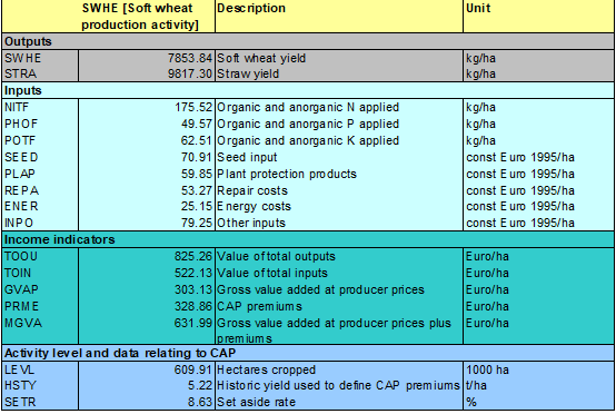
The economic activities in the agricultural sector are broken down conceptually into ‘production activities’ (e.g. cropping a hectare of wheat or fattening a pig). These activities are characterised by physical output and input coefficients. For most activities, total production quantities can be found in statistics and output coefficients derived by division of activity levels (e.g. ‘soft wheat’ would produce ‘soft wheat’ and ‘straw’, whereas ‘pigs for fattening’ would produce ‘pig meat’ and NPK comprised in manure). However, for some activities other sources of information are necessary (e.g. a carcass weight of sows is necessary to derive the output coefficient for the pig fattening process). For manure output engineering functions are used to define the output coefficients. The way the different output coefficients are calculated is described in more detail below.
The second part characterising the production activities are the input coefficients. Soft wheat, to pick up our example again, would be linked to a certain use of NPK fertiliser, to the use of plant protection inputs, repair and energy costs. All these inputs are used by many activities, and official data regarding the distribution of inputs to activities are not available. The process of attributing total input in a region to individual activities is called input allocation. It is methodologically more demanding than constructing output coefficients. Specific estimators are developed for young animals, fertilisers, feed and the remaining inputs, which are discussed below.
Multiplied with average farm gate prices for outputs and inputs respectively, output coefficients define farm gate revenues, and input coefficients variable production costs. The average farm prices used in the CAPRI data base are derived from the EEA and hence link physical and valued statistics. However, in some cases as young animals and manure which are not valued in the EEA, own estimates are introduced.
In order to finalise the characterisation of the income situation in the different production activities, subsidies paid to production must be taken into account. The CAPRI data base features a rather complex description of the different CAP premiums allocated to the individual activities. However, subsidies outside of the CAP for the EU Member States have received less attention (in line with smaller amounts).
The following table gives an example for selected activity related information from the CAPRI data base.
Table 1: Example of selected data base elements for a production activity
Technology variants for production activities
For most activities there are two technologies available, typically a low and a high yield variety. Usually they are defined to cover each 50% of the activity level observed in ex post data, but with some particularities in the sugar sector (see ‘/sugar/techf.gms’).
Linking production activities and the market
The connection between the individual activities and the markets are the activity levels. Total soft wheat produced is the sum of cropped soft wheat hectares multiplied with the average soft wheat output coefficient. In cases like pig meat, as mentioned before, several activities are involved to derive production.
The produced quantities enter the farm and market balances. Production plus imports as the resources are equal to the different use positions as exports, stock changes, feed use, human consumption and processing. These balances are only available at Member State, not at regional level. Production establishes the link to the EAA as well, as average farm gate prices are unit values derived by dividing the values from the EAA by production quantities.
The three basic identities linking the different elements of the data base are expressed in mathematical terms as following. The first equation implies that total production or total input use (code in the data base: GROF or gross production/gross input use at farm level) can be derived from the input and output coefficients and the activity levels (LEVL):
\begin{equation} GROF_j = \sum_j{LEVL_j \cdot IO_j} \end{equation}
The second type of identities refers to the farm and market balances:
\begin{align} \begin{split} GROF_{io}-SEDF_{io}-LOSF_{io}-INTF_{io} &=NETF_{io}\\ NETF+IMPT_{io} &=EXPT_{io}+STCM_{io}\\ &\quad+FEDM_{io}+LOSM_{io}\\ &\quad+SEDM_{io}+HCOM_{io}\\ &\quad+INDM_{io}+PRCM_{io}\\ &\quad+BIOF_{io} \end{split} \end{align}
The farm balance positions are seed use (SEDF) and losses (LOSF) on farm (only reported for cereals) and internal use on farm (INTF, only reported for manure and young animals). NETF or net trade on farm is hence equal to valued production/input use and establishes the link between the market and the agricultural production activity. Adding imports (IMPT) to NETF defines total resources, which must be equal to exports (EXPT), stock changes (STCM), feed use on market (FEDM), losses on market (LOSM), seed use on market (SEDM), human consumption (HCOM), industrial use (INDM), processing (PRCM), and use for biofuel production (BIOF).
The third identity defines the value of the EAA in producer prices (EAAP) as sold production or purchased input use (NETF) in physical terms multiplied with the unit valued price (UVAP):
\begin{equation} EAAP_{io}=UVAP_{io}NETF_{io} \end{equation}
The following table shows the elements of the CAPRI data base as they have been arranged in the tables of the data base.
Table 2: Main elements of the CAPRI data base
| Activities | Farm- and market balances | Prices | Positionsform from the EAA | |
|---|---|---|---|---|
| Outputs | Output coefficients | Production, seed and feed use, other internal use, losses, stock changes, exports and imports, human consumption, processing | Unit value prices from the EAA with and without subsidies and taxes | Value of outputs with or without subsidies and taxes linked to production |
| Inputs | Input coefficients | Purchases, internal deliveries | Unit value prices from the EAA with and without subsidies and taxes | Value of inputs with or without subsidies and taxes link to input use |
| Income indicators | Revenues, costs, Gross Value Added, premiums | Total revenues, costs, gross value added, subsidies, taxes | ||
| Activity levels | Hectares, slaughtered heads or herd sizes | |||
| Secondary products | Marketable production, losses, stock changes, exports and imports, human consumption, processing | Consumer prices |
The Complete and Consistent Data Base (COCO) for the national scale
The COCO database is built by the application of two modules:
COCO1 module:
Prepare national database for all EU27 Member States the Western Balkan Countries, Turkey and Norway.
It is basically divided into three main parts:
- A data import “part” that is not a single “module” but rather a collection activity to prepare a large set of very heterogeneous input files
- Including and combining these partly overlapping input data according to some hierarchical overlay criteria, and
- Calculating complete and consistent time series while remaining close to the raw data.
Data preparation (part 1) and overlay (part 2) form a bridge between raw data and their consolidation to impose completeness and consistency. The overlay part tries to tackle gaps in the data in a quite conventional way: If data in the first best source (say a particular Eurostat table from some domain) are unavailable, look for a second best source and fill the gaps using a conversion factor to take account of potential differences in definitions. To process the amount of data needed in a reasonable time this search to second, third or even fourth best solutions is handled as far as possible in a generic way in the GAMS code of COCO where it is checked whether certain data are given and reasonable. However there are a few special topics that are explained in separate sections.
COCO2:
The finishing step estimates consumer prices, consumption losses, and some supplementary data for the feed sector (by-products used as feedstuffs, animal requirements on the MS level, contents and yields of roughage). Both tasks run simultaneously for all countries and build on intermediate results from the main (COCO1) part of COCO like human consumption and processing quantities.
Overview and data requirements for the national scale
An overview on the key data collection, assingments and corrections in main program coco1.gms is given in the following figure.
Figure 2: Overview on key elements in the consolidation of European data at the Member state level (in coco1.gms)
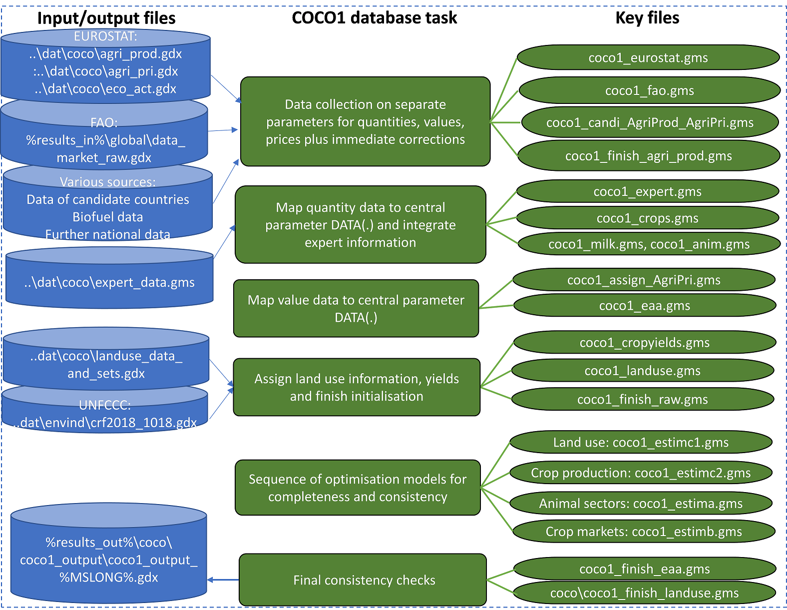
Source: Own illustration
The different steps will be explained in more detail in the following sections.
The CAPRI modelling system is, as far as possible, fed by statistical sources available at European level which are mostly centralised and regularly updated. Farm and market balances, economic indicators, acreages, herd sizes and national input output coefficients were initially almost entirely from EUROSTAT. In the course of time, more and more special data sets have been added to fill gaps or resolve problems detected in EUROSTAT data, such as specific data on Western Balkan Countries or on the biofuel sector.
The main sources used to build up the national data base are shown in the following.
Table 3: Data items and their main sources
| Data items | Source |
|---|---|
| Activity levels | Eurostat: Crop production statistics, Land use statistics, herd size statistics, slaughtering statistics, statistics on import and export of live animals For Western Balkan Countries and Turkey: Eurostat supplemented with national statistical yearbooks, data from national ministries, FAOstat production statistics and others |
| Production, farm and market balance positions | Eurostat: Farm and market balance statistics, crop production statistics, slaughtering statistics, statistics on import and export of live animals For Western Balkan Countries and Turkey: Eurostat supplemented with national statistical yearbooks, data from national ministries, FAOstat production statistics and others |
| Sectoral revenues, costs, and producer prices | Eurostat: Economic Accounts for Agriculture (EAA) and price indices for gap filling, otherwise unit value calculation For Western Balkan Countries and Turkey: Supplemented with national statistical yearbooks, data from national ministries, results from AgriPolicy, FAOstat price statistics |
| Consumer prices | Derived from macroeconomic expenditure data (Eurostat, supplemented with UNSTATS) and food price information from various sources |
| Output coefficients | Derived from production and activity levels, engineering knowledge |
Data Import
A large set of very heterogeneous input files (in terms of organisation and format) is collected, currently covering the following years:
Table 4: Temporal coverage of national data by region
| Member State | Range |
|---|---|
| EU15 Member States without Germany | 1984 – 2018/2019 |
| Germany and (12) New Member States | 1989 – 2018/2019 |
| Western Balkan (WB) Countries and Turkey | 1995 – 2018/2019 |
| Norway | 1984 – 2017 |
Eurostat data
First step: Data download and format conversion Data are originally downloaded in “TSV-format”, as offered by Eurostat for bulk data users. The TSV-format is a flat file format for time series. Data can be selected for all EU MS and some Candidate Countries. Availability differs by country, of course (almost nothing for the Kosovo, Montenegro, Bosnia & Herzegonina). In the process of downloading the TSV files are also converted in GAMS readable form (csv or gdx). The following themes and table groups of Eurostat are accessed:
Agriculture, forestry and fisheries
- Agriculture (“agr”)
- Economic Accounts for Agriculture (Table Group “aact”, saved on CAPRI parameter “p_ecoact”
- Agricultural prices and price indices (Table Group “apri”, saved on CAPRI parameter “p_agripri”
- Agricultural product related physical information (production, activity levels from Table Group “apro”, saved on CAPRI parameter “p_agriprod”
- Older, discontinued Eurostat series that still provide useful information (requiring some ad hoc extrapolations), for example (a) market balance information for products other than cereals, oilseeds and wine, critical for “COCO1”, (b) relative price level indices of food products (MS relative to EU average) for COCO2, © availability and production of feedingsstuffs (useful for COCO2 completions on feed from by-products)
Economy and Finance
- National annual accounts (“nama10”)
- Annual national accounts → National Accounts detailed breakdowns (by industry, by product, by consumption purpose) → Final consumption expenditure of households by consumption purpose (COICOP 3 digit),
- General indicators to National Accounts - Population and employment
- GDP and main components - Current prices, volumes, price indices
- Prices (“prc”)
- Harmonized indices of consumer prices (prc_hicp) here: HICP (2005=100) -annual Data, and HICP - Item weights
Second step: data selection and code mapping
The second step is data selection and code mapping performed by the GAMS program ‘coco_input.gms’. Cross sets linking Eurostat codes to COCO codes define the subset of data series subsequently used.
The mapping rules are collected in two sub-programs called by ‘coco_input.gms’, for example:
- ‘gams/coco/ eurostat_agriculture_mapping.gms’ for the tables from Eurostat’s “Agriculture and Fisheries” Statistics
- ‘eurostat_ econfinc_mapping.gms’ for the tables from Eurostat’s “Economy and Finance” Statistics
Example from file ‘Eurostat _agriculture_mapping.gms’. The results of the program run are gdx-files loaded by files (e.g. coco/coco1_eurostat.gms) which are in turn loaded by coco1.gms or coco2.gms.
<html> <head> <META http-equiv=Content-Type content=“text/html; charset=UTF-8”> <title>Exported from Notepad++</title> <style type=“text/css”> span {
font-family: 'Consolas';
font-size: 9pt;
color: #000000;
} .sc0 { } .sc9 {
font-weight: bold;
color: #0000FF;
} .sc12 {
font-weight: bold;
color: #6600CC;
} .sc13 {
font-weight: bold;
color: #6600CC;
} .sc16 {
color: #880000;
} .sc24 { } </style> </head> <body> <div style=“float: left; white-space: pre; line-height: 1; background: #FFFFFF; ”><span class=“sc9”>SET</span><span class=“sc24”> </span><span class=“sc0”>EcoActMAP</span><span class=“sc13”>(</span><span class=“sc0”>ASS_COLS</span><span class=“sc12”>,</span><span class=“sc0”>ASS_ROWS</span><span class=“sc12”>,</span><span class=“sc0”>eco_act_ori_eurostat</span><span class=“sc13”>)</span><span class=“sc24”> </span><span class=“sc16”>“mapping”</span><span class=“sc24”> </span><span class=“sc12”>/</span><span class=“sc24”> </span><span class=“sc0”>EAAP.CERE.</span><span class=“sc24”> </span><span class=“sc0”>aact_eaa01_01000_PROD_PP_MIO_EUR</span><span class=“sc24”> </span><span class=“sc0”>EAAP.SWHE.</span><span class=“sc24”> </span><span class=“sc0”>aact_eaa01_01110_PROD_PP_MIO_EUR</span><span class=“sc24”> </span><span class=“sc0”>EAAP.DWHE.</span><span class=“sc24”> </span><span class=“sc0”>aact_eaa01_01120_PROD_PP_MIO_EUR</span><span class=“sc24”> </span><span class=“sc12”>/;</span><span class=“sc24”>
</span><span class=“sc9”>SET</span><span class=“sc24”> </span><span class=“sc0”>AgriProdMAP</span><span class=“sc13”>(</span><span class=“sc0”>ASS_COLS</span><span class=“sc12”>,</span><span class=“sc0”>ASS_ROWS</span><span class=“sc12”>,</span><span class=“sc0”>agri_prod_ori_eurostat</span><span class=“sc13”>)</span><span class=“sc24”> </span><span class=“sc16”>“mapping”</span><span class=“sc24”> </span><span class=“sc12”>/</span><span class=“sc24”> </span><span class=“sc0”>CERE.LEVL.</span><span class=“sc13”>(</span><span class=“sc24”> </span><span class=“sc0”>apro_cpnh1_C1000_AR</span><span class=“sc12”>,</span><span class=“sc0”>apro_cpnh1_h_C1000_AR</span><span class=“sc13”>)</span><span class=“sc24”> </span><span class=“sc0”>SWHE.LEVL.</span><span class=“sc13”>(</span><span class=“sc24”> </span><span class=“sc0”>apro_cpnh1_C1110_AR</span><span class=“sc12”>,</span><span class=“sc0”>apro_cpnh1_h_C1110_AR</span><span class=“sc13”>)</span><span class=“sc24”> </span><span class=“sc0”>SWH1.LEVL.</span><span class=“sc13”>(</span><span class=“sc24”> </span><span class=“sc0”>apro_cpnh1_C1111_AR</span><span class=“sc12”>,</span><span class=“sc0”>apro_cpnh1_h_C1111_AR</span><span class=“sc13”>)</span><span class=“sc24”> </span><span class=“sc12”>/;</span><span class=“sc24”>
</span></div></body> </html>
Western Balkan Countries and Turkey
For those countries Eurostat data need completion in almost every area which is handled in country specific xls files. The structure of these supplementary Excel country sheets and the definitions of the data are tailored to COCO. The resulting sheets in these xls files are uniform across countries, in order to ease data extraction for the modelling part by applying macros. However, each national information system has its own peculiarities and hence, not all data are fully harmonised across countries. Various sources are assessed and combined in a case by case manner: Eurostat data, if already available and plausible, are handled as the preferred data source. Data collected from the national statistical yearbooks have second priority, followed by expert data collected in from earlier projects. Finally FAO data provides often the fall-back solution for any remaining missing time series.
The final sheet in each of these country specific xls files is the interface to the GAMS programing world of COCO. An Excel macro “SELECT_data_all” collects the time-series compiled in other sheets and puts them into this final sheet with the appropriate COCO code. Another macro finally exports the numbers into text files like “dat/coco/bosnia_coco.gms”. Because the xls file are quite complex due to various linkages, we do not read directly from them. This avoids unplanned changes and permits convenient tracing of data changes via the CAPRI versioning system svn.
Supplementary data for Romania and Bulgaria
Country level data from national experts were compiled in Excel files that help in particular to complete the meat and milk sectors.
FAO data selection
Two FAO data sources are combined:
- For all regions FAO data (mapped in the context of module “global database” to CAPRI codes and hence consistent across modules) serve as a fall back option under certain conditions, defined in the code. This fall back function of FAO data has gained in importance since Eurostat discontinued the publication of most market balances since 2014. In some cases also activity level (area) information may be taken from FAO.
- Some particular data like disaggregate data on herds of chicken, ducks, turkeys and geese are compiled in a separate include file dat/coco/fao_add.gms because these data types are usually not loaded for global database.
Other additional input data
COCO1: Biofuels
- Production, market balance and feedstock quantities for biodiesel and bioethanol are collected from a multitude of sources:
- EU project www.elobio.eu (production, demand, biodiese and bioethanol, 1999-2007)
- Eurostat, Energy balances and demand (tables nrg_xxxx) production, demand, trade for diesel, gasoline, biodiesel and bioethanol, 2001-15)
- Eurostat, Production and trade (PRODCOM), ethanol and biodiesel, 2000-14
- PRIMES model1) database (production, biodiesel and bioethanol, 2000-07)
- US Energy Information Administration (EIA), production of biodiesel and bioethanol, 2000-12, incl. some non-EU countries
- DG Agri Ethanol balances (production partly with split by feedstocks and MS, demand and trade)
- Aglink ex post database (most data for Turkey, also EU biofuel production from non-standard sources (NAGR).
- USDA GAIN reports (market balances for Serbia, feedstocks for biodiesel in EU)
- FAOstat (market balances for palm oil)
- Prices at the pump and retail prices for diesel and gasoline are from Eurostat’s energy database (http://epp.eurostat.ec.europa.eu/portal/page/portal/energy/data/database), supplemented with IEA Statistics 2016 for Turkey.
- Taxes for diesel, gasoline, biodiesel and bioethanol are collected from DG Energy website and publications, and EURACTIV, EU news & policy debates, Brussels (http://www.euractiv.com/en/enterprise-jobs/fuel-taxation/article-117495)
- Some supplementary Aglink data give information on feedstock composition, tariffs and world market prices for crude oil, biodiesel and bioethanol.
- Trade data for undenatured ethyl alcohol, denatured ethyl alcohol, fatty acid mono-alkyl esters, crude palm oil, palm and fraction and palm kernel and fraction are collected from Eurostat’s COMEXT data (2000-14).
- Market balances for palm oil are taken from FAOstat and supplemented with COMEXT.
COCO1: Sugar Quotas
- All sugar quotas 1999 until 2006 from the annual sugar yearbook.
- Buy-back 2006 in the restructuring program from CAP monitor 16 January 2008.
- Sugar quotas renounced by member states following sugar reform (2006-2010), information from Wirtschaftliche Vereinigung Zucker e.V. (WVZ) and Verein der Zuckerindustrie e.V. (VdZ), Bonn (http://www.zuckerwirtschaft.de/1_3_2_1.htm) and KWS SAAT AG, Einbeck (http://www.kws.de/ca/fh/thd/)
COCO1: Milk
- Market balances for casein and whey powder were only available on EU level from ZMP, Bonn, which was closed down in 2009.
- DG Agri partly completes gaps in Eurostat series and offers this consolidated database for download. This is used to close gaps in gams/coco/coco1_eurostat.
COCO1: Producer prices for cotton
Import unit values for cotton seeds, cotton lint, flax and hemp are additionally selected from COMEXT.
COCO1: Expert data
Data from experts, which will overwrite all Eurostat data, is included for special issues for some Member States (e.g. grass yields for the Netherlands).
This also applies at the moment for all Norwegian input data such that Eurostat data are currently ignored. However, as Eurostat completeness has also improved on Norway, this procedure might be reconsidered in the future.
COCO1: Land use data
The raw data on land use are currently prepared outside the CAPRI system. Source code and input files are available at EuroCARE, Bonn (R:/Coco_input/land_use). Relevant (raw) information is stored in dat/coco/landuse_data_and_sets.gdx. The data base comprises information on land use classes from various sources, which are again partly discontinued but useful for the early years:
- REGIO - Eurostat, land use, REGIO domain( NUTS2 level - yearly, 1984-2014)
- ENVIO - Eurostat, land use, env_la_luc1.xls (MS level - 1985, 1990,1995, 2000)
- LANDCOVER - Eurostat, land cover(MS level – 2009, 2012, 2015)
- Corine Land Cover (CLC), 44clc_nuts2.xls (NUTS2 level - 1990, 2000, 2006, 2012)
- FAO - area.xls(MS level - yearly, 1984-2016)
- MCPFE (Ministerial Conference on the Protection of Forests in Europe), jointly published by FAO and UNECE (MS level - 1990, 2000, 2005, 2010, 2015)
- FSS - Eurostat, FSS(NUTS2 level - 1990, 1993, …, 2007, 2010, 2013), only added in coco1/landuse
- UNFCCC (1990-2016), also covers land transitions and settlement data. Official data for LULUCF accounting, merged with other data in coco1_landuse.
COCO2: Economic data
- Eurostat: Economy and Finance, Exchange rates, Bilateral exchange rates, Euro/ECU exchange rates. Data is already prepared in Excel for premature introduction of Euro in price data from the International Labour Organisation (ILO).
- Eurostat, population. To complete early years data from and old Eurostat domain (AGRIS, Population) are also loaded.
- GDP price index expressed in Euros
COCO2: Expenditures
Consumer expenditures on food items are included from:
- Eurostat: Old domain SEC2 for data up to 1997 (HIST)
- Instituto Nacional de Estadística m(INE): Anuario de Estadística Agroalimentaria (AEA), Consumer expenditure on food items in Spain close to HIST definitions up to 1996
- Rheinisch-Westfälisches Institut für Wirtschaftsforschung (RWI): Consumer expenditure on food items for DEW 1985-92 in Mio DM
- Statistisches Bundesamt Deutschland (SBA): Weighted average of expenditure shares in German household types 2 and 3 (1985-91)
- Eurostat, Final consumption expenditure of households by consumption purpose (COICOP 3 digit)
- United Nations Statistics Division (UNSTATS): Household consumption expenditure in USD
- Eurostat, PRICE: Consumer expenditure weights are used as indicators for budget shares
- Eurostat: Economy and Finance, GDP and main components, Final consumption expenditure of households: Total private consumption of households in current prices (Table “a_gdp_c”)
COCO2: Consumer food prices and consumer food price indices
Food price indices from:
- Eurostat, PRICE, 2005=100.
- Several national sources for western Balkan regions
- Eurostat: Old domain FOOD of section AGRICULTURE: Aggregate food price index with old Eurostat methodology and base 1985
- INTERNATIONAL LABOUR ORGANIZATION Geneva (ILO): LABORSTA Labour Statistics Database, retail prices of selected food unit, prices indices of selected food unit, discontinued after 2008
- Eurostat: Detailed average prices – 2008 - 2015 [table prc_dap15] is used to extend the ILO consumer price series.
COCO2: By-products
- FAO: Food Balance Sheets, Commodity Balances, Livestock and Fish Primary Equivalents: Imports and exports quantities for fish meal, dried cassava, gluten deed and meal, as well as feed quantities for fish meal.
- Eurostat: Purchase prices for fish meal, dried sugar beet pulp, soya cake, and wheat bran
- Eurostat: data (at most up to 2010) from discontinued tables (“food_in afeed1” and “bilares”) on production of feedingstuffs and availability of feedingstuffs
- FAO: Food Balance Sheets, Commodity Balances, Crop Primary Equivalents: Milled rice and total sugar unit value
- Netherlands Economic Institute (NEI): Purchase prices for sugar, calculated by the average of Intervention Price and CAOBISCO price
COCO2: Milk Products
- Zentrale Markt- und Preisberichtstelle (ZMP): Producer prices of selected milk products (only available for some countries)
- Agrarmarkt Informations-Gesellschaft mbH (AMI): AMI-Marktbilanz Milch 2011 (only available for some countries)
- DG AGRI (Réponses au questionnaire (art. 8 du Règlement (CEE) n° 536/93), (art. 15 R 1392/2001) and (art. 26 R 595/2004)): Data on direct sales of raw milk and farm processing in DG AGRI definitions for quota administration
COCO2: Others
- Eurostat: External trade, External trade detailed data, COMEXT, EU27 Trade Since 1988 By CN8, Reporter EU15: Auxiliary trade data for wheat, soft wheat and durum wheat, export values and quantities for cotton and cotton seeds, data on imports and exports of most relevant by-products
- Statistisches Jahrbuch ueber Ern., Landw. U. Forsten, 1999, 2006 und 2010 (Aufkommen u Verbrauch von Futtermitteln): Net imports and feed from domestic production of by-products in Germany
- USDA: Prices for soya, rape and sunflower cake and oil, prices for corn gluten feed
COCO1: Overlay from various sources
The main program coco1.gms starts with a number of declarations of sets and parameters to handle the collection and overlay of “raw data”, often given in a classification different from the target one (sets COLS, ROWS).
 A recurrent characteristic of COCO is to solve the problem: if the first best source has gaps in a particular country, or even is entirely empty, select the second or even third best source to fill the gaps.
Including standard and supplementary data from Eurostat (‘coco1_eurostat.gms’)
The main program coco1.gms proceeds by importing data from Eurostat prepared beforehand (in coco_input.gms). The main data (on p_agriProd, p_ecoAct, and p_agriPri) are processed step by step and corrections made on selected data for all MS2).
Data from FAOstat (‘coco1_fao.gms’)
The general fall-back option for missing data is FAOstat which requires a few corrections compared to the standard mappings in the context of module “global database”, including:
- Rebooking of “other use” to processing (PRCM) or other balance positions
- Disaggregation of olives (table olives, olives for oil), grapes (table grapes, grapes for wine), wheat (common, durum)
- Checks for data changes after sugar reform 2006
- Country specific fixes like in coco1_eurostat.gms.
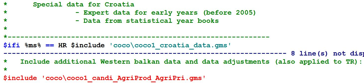
Data from additional sources for the Western Balkan Countries and Turkey (‘coco1_croatia_data.gms’ and ‘coco1_candi_AgriProd_AgriPri.gms’)
Croatia is the first country singled out from the special data input for the Western Balkan Countries and Turkey. Croatia is by now mostly sourced from Eurostat, as the other EU members, but a few supplementary expert data have been retained. For the other Western Balkan regions and Turkey, ‘coco1_candi_AgriProd_AgriPri.gms' further adapts the WB data from the country specific xls files to match the COCO definitions that also apply to EU28 countries (on parameters p_agriProd and p_agriPri).
The include file handles the following:
- Similar to EU-28 MS there are many case-by-case adjustments correcting different scaling and definitions (live weight ↔ carcass weight, reaggregations for wine and fruits…).
- In many cases, market balances are simply incomplete. As a fall back solution, domestic demand is calculated from production and net trade and disaggregated with shares taken from a sister country aggregate (Romania, Bulgaria, Greece, Slovenia, Hungary). Other corrections with “borrowed” information are:
- Trade data are frequently missing in the WBs, such that FAO data are included where available.
- Production of oilcakes and sugar is estimated from raw products, if missing, using the sister country aggregate processing coefficients;
- The production of milk products is estimated from processing coefficients in Serbia which has a quite complete series;
- Price information is also completed relying on the sister country aggregates.
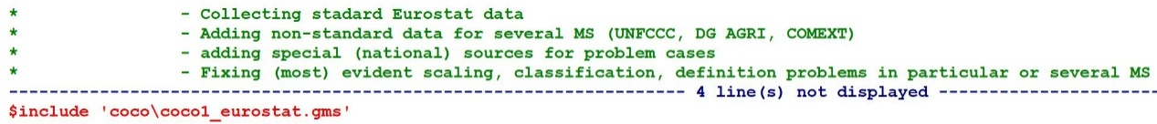
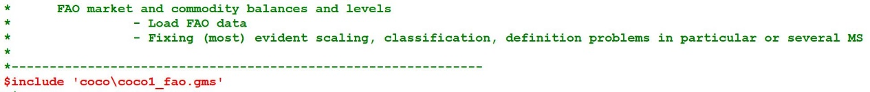
Final completions and revisions for all Member States (‘coco1_finish_agriprod.gms’)
Based on the availability of second and third best options various finalising steps are applied to the quantity data. It should be noted that the CAPRI database tries to estimate market balances (needed for separate behavioural function for feed, food, processing, biofuel demand) in spite of Eurostat discontinuing the publication of market balances for most products since 2014. For this purpose the old Eurostat market balances are still loaded and combined with more recent production data. This triggers the need for data completions and estimations in the most recent years (which are also most critical for projections). In 2019 market balance data have returned to the Eurostat server for cereals and oilseeds, but only for a single year (2017) ⇒ It is likely that adjustments like the following will also be needed in the future:
- Completion of production data from the (discontinued) Eurostat market balance statistics (model code “USAP”) with quantity information given from the production statistics (code “GROF”) or from agricultural account statistics (model code “EAAQ”) using a correction factor calculated from overlapping years.
- Additional gap filling using FAO data for special cases and general cases of missing data (e.g. for balances). An additional difficulty is that FAO commoditiy balances are currently (2019) also ending in 2013 (especially valuable for recent years).
- Domestic use can be calculated (under some conditions) from imports, export and usable production. If only domestic use is given for some products, the sub-positions, such as industrial use, processing, human consumption, feed on market, total seed and total losses are allocated with the average shares in data for other years, from the same country. As a fall back solution, the average shares from other countries are used.
- For the milk products whey powder and casein, the disaggregation of demand is mainly based on EU data collected by the German “Zentrale Markt- und Preisberichtstelle für Erzeugnisse der Land-, Forst- und Ernährungswirtschaft GmbH” (ZMP) and some auxiliary assumptions.
- As data for oilseeds are critical for all countries, the implied processing coefficient is checked for plausibility. If the national coefficient is lower than 60% or above 150% the average coefficient for all EU-15 MS, the data for usable production of the country are corrected by multiplying the processing data with the average EU-15 coefficient. Domestic use and all sub-positions are subsequently re-calculated.
- Some additional calculations to prepare the use of animal herd data in coco1_anim:
- Some calculations to combine FAO and FSS data on poultry herds
- Completions acknowledging seasonality in cattle and sheep and goats herd countings
- Aggregations and residual calculations to the COCO animal categories from animal types in Eurostat (say “Heifers for raising, 1-2 years”)
The file handling the previous actions is ‘coco1_finish_agriprod.gms’:
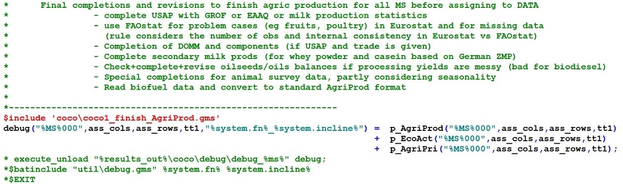
The previous code snippet also shows for the interested reader two frequently used debugging devices:
- The key parameters at a certain point in the program flow (above: p_agriProd, p_agriPri, p_ecoAct) are copied to a debugging parameter “debug” (better name would be: “p_debug”). At the end of a coco1 run (or if desired also at this point) the parameter is unloaded into a file “results/coco/debug/debug_%MS%.gdx” such that the various assignments, corrections, deletions that have occurred up to a certain program line may be inspected in one file.
- The next command “$batinclude “util/debug” %system.fn% %system.incline% unloads the whole memory, incuding all parameters but also sets and other symbols, at this point into a debugging file in the gams/temp folder. This may be useful to analyse “difficult” cases of debugging.
Finally the biofuel sector is prepared.
EU biofuel sector data (‘coco1_finish_agriprod.gms’ and ‘prepare_biofuel_data.gms’)
The first issue to note is that market balances for sugar beet and sugar are compiled in such a way that all biofuel use of beets is converted into biofuel use of sugar, as if the beets were first processed to sugar and only then converted to ethanol. The advantage of this approach is that sugar is part of the market model and thus may enter the behavioural functions for biofuel feedstock use whereas beets only exist in the supply part of CAPRI. A second advantage is that biofuel feedstock use was indeed booked under sugar in some MS and under beets in others such that our approach ensures a standardisation of booking principles.
Biofuel production
There is no differentiation made between fuel- or non-fuel (undenatured or denatured) quantities in production, import and export positions of ethanol. But the consumption position of ethanol is differentiated in fuel-ethanol consumption and non-fuel-ethanol consumption. Hence data on fuel and non-fuel production and consumption of ethanol was required. In the case of biodiesel this differentiation is irrelevant. The ex-post data on biofuel production are coming from diverse sources which is unavoidable to complete the data for years as of 2002 up to the present, if necessary with the help of second and third best solutions or assumptions (compare biofuel/prepare_biofuel_data.gms).
The overlay considers data availability and consistency across sources:
- For ethanol we consider DG agri as the first best source as it does not only cover production and demand, but also a break down by feedstocks (cereals, beets, wine, fruits, potatoes, other).
- Some countries (Croatia, Turkey, Bulgaria, Romania, Serbia) are supplemented from other sources (AGLINK-COSIMO, USDA, Eurostat PRODCOM). AGLINK also supplements production other than from agricultural feedstocks.
- Eurostat PRODCOM, Energy balances and PRIMES serve to extrapolate or backcast the DG Agri information to years with missing data.
- Ethanol trade by MS is taken from COMEXT but scaled to be in line with DG AGri data for the whole EU.
- Production of biodiesel is usually from the energy balances while trade is from COMEXT. If data are complete and results reliable, demand is computed residually. In cases of missing data or implausible results, demand is taken from Energy balances, PRIMES, or the EloBio project and trade is calculated as a residual with some rules.
Feedstock demand
In addition to market balances for the fuels the CAPRI data base requires the shares of the raw products on the production of biodiesel and bioethanol at the level of CAPRI products. For bioethanol, this information is partly provided by the DG Agri balances, hence this has been selected to be the major source. The detailed recording follows from the existence of support measures for distillation of wine, fruits and potatoes which triggered a detailed monitoring of ethanol markets. However, for biodiesel the statistical sources are scarce. It turns out that the most consistent estimates for EU regions are apparently produced by USDA services, covering rape, sunflower, soya, palm oil but also used cooking oils, tallow and other oils. As these data do not cover single MS an estimation procedure has been devised (in biofuel/calc_feedstock_shares.gms). The initialisation of this estimated feedstock composition relied on the observed increase in INDM according to Eurostat (or more precisely the COCO initialisation when entering ‘prepare_biofuel_data.gms’) which is assumed to be the main source to “cut out” the required biofuel processing quantities (BIOF) by MS from market balances that so far did not include BIOF.
A special case was palm oil, as the CAPRI database (COCO) doesn’t cover an industrial use position for this product so far. EUROSTAT-COMEXT delivers data on import and export quantities of crude palm oil (HS 151110) for EU Member states. Thereby an increase of palm oil imports was observed within the relevant ex post period (2002-2005). Thus the following assumptions were made to derive approximated values for palm oil processing to biodiesel: (a) Import quantities minus export quantities are equal to domestic consumption of palm oil as domestic production in European Member states can be neglected. (b) The average aggregated consumption quantity of palm oil before 2002 was assumed to be completely used for human consumption as no significant biodiesel consumption took place. By subtracting this constant share of human consumption from the observed consumption quantities after 2002 gave an estimate for the quantities used for industrial processing
Given that many data sources are combined and several aggregation conditions should be maintained, it turned out necessary to set up a small optimisation problem with the following properties (see towards the end of ‘prepare_biofuel_data.gms’):
- The estimation tries to stay close to the initial feedstock composition
- Extra terms penalise deviations from DG Agri (first best souce for ethanol) and implausibly high shares for palm oil
- Technical conversion coefficients (see below) link standard feedstock use and estimated production which has to aggregate with non-standard feedstocks (NAGR) to total production of biofuels. Non-standard feedstocks are those not endogenous in the CAPRI market model (potatoes, fruits and other for bioethanol, used cooking oils, tallow and other for biodiesel)
- Total domestic use (with data modifications heavily penalised in the objective) is consistently broken down into biofuel use, other industrial use and non-industrial (e.g. food) use to avoid disturbing the initialisation in previous include files based on Eurostat data.
Technology parameters
Conversion coefficients for 1st generation biofuels were collected from different sources. The AgLink-Cosimo model includes a set of conversion coefficients which are in line with the CAPRI product definitions and have become the main source for CAPRI. The table below displays the set of conversion coefficients used for 1st generation biofuels and corresponding by-products.
Table 5:Conversion coefficients for 1st generation biofuel production
| Conversion coefficients (t/t) | Ethanol | Byproducts | |
|---|---|---|---|
| Grains | Wheat | 0.274 | 0.266 DDGS |
| Barley | 0.247 | 0.266 DDGS | |
| Oats | 0.247 | 0.266 DDGS | |
| Rye | 0.247 | 0.266 DDGS | |
| Corn (dry milling) | 0.335 | 0.292 DDGS | |
| Other | Table Wine | 0.100 | |
| Sugar Crops | Sugar | 0.517 | |
| Sugar beets | 0.079 | 0.004 Vinasses* | |
| Biodiesel | Byproducts | ||
| Veegetable oils | Rape oil | 0.922 | 0.100 Glycerine |
| Soy oil | 0.922 | 0.100 Glycerine | |
| Sunflower oil | 0.922 | 0.100 Glycerine | |
| Palm oil | 0.922 | 0.100 Glycerine | |
Note: The beet coefficient has been increased in the meantime from 0.079 to 0.086.
Fuel prices and taxes
For a specification of processing-, biofuel supply- and demand-functions in the base year, ex post prices are required. Furthermore, given the structure of the CAPRI market module (described in Section Market module for agricultural outputs ), a differentiation of producer, consumer and import price is also needed. These differentiated prices are not covered in any statistical database for biofuels but they can be derived indirectly by given information on taxes, tariffs and subsidies from the world market price which is available. Thus beside ex post prices information on consumer (excise) taxes, import tariffs and further subsidies are required. The AgLink-Cosimo database includes ex post world market prices for ethanol and biodiesel. This price was taken as the base value to calculate the differentiated prices in the respective countries. The import tariffs for ethanol and biodiesel were also taken from the AgLink-Cosimo database. As the consumer taxes for ethanol and biodiesel in most instances correspond to a reduced excise tax on fossil fuels the consumer taxes for gasoline and diesel were taken as a base value. This tax information was acquired from EurActiv3) where levels of diesel and petrol taxation in 2002 are published for European Member states. For the required time period (2002-2005) taxation levels were calculated with respect to COM(2002)4104) which set minimum excise tax rates for non-commercial diesel and petrol since 2006. To identify the excise tax exemptions and producer subsidies, if existent, for the single Member states the obligatory ‘Member States reports on the implementation of Directive 2003/30/EC of 8 May 2003 on the promotion of the use of biofuels or other renewable fuels for transport’ were consulted which are published by the Commission5). Three different types of tax regulations for biofuels were identified which are applied among the different Member states: an absolute tax for biofuels, an absolute reduction of the excise tax on fossil fuels and a relative reduction of the excise tax on fossil fuels. All differentiated in taxation for blended biofuels or pure biofuels. Based on this information the different ex post prices for the period 2002-2005 were recalculated. As the envisaged biofuel demand function will be a function of (among other variables) the relation between fossil fuel consumer prices and biofuel consumer prices the acquisition of fossil fuel prices was required additionally. To hold consistency between the biofuel and fossil fuel prices the price information for fossil fuels were also taken from the AgLink-Cosimo database which provides EU market prices for diesel and petrol. For the recalculation of consumer prices in individual Member states the already collected taxation levels for fossil fuels were applied. Because there exists a significant difference between the physical energy content and the density of biodiesel, ethanol, petrol and diesel a direct comparison of prices (in €/t) is not possible. For this reason the prices as well as the taxation levels were converted into Euro per ton oil equivalent (toe).
Assigning data to database array
So far data processing has focussed on the key Eurostat Table Group “apro” (collected on parameter p_agriProd). The next parts of COCO will collect data from other sources, including the other two Table Groups for prices and Economic accounts (“apri”, “aact”) to a single GAMS array “data”. This data collection activity happens in files coco1_expert.gms to coco1_eaa.gms with a summary of the details given below.

Include file ‘coco1_expert.gms’
This file collects expert data for specific countries that receive priority over all other data sources in the initialisaiton. The most relevant case is Norway where nearly all data are provided and checked by NIBIO (Norwegian Institute of Bioeconomy Research).
Include file ‘coco1_crops.gms’
This sub-module assigns the areas, crop production data and most market balance positions from Eurostat’s Table Group “apro” . However, it is necessary to first deal with a double counting in the land use statistics of Eurostat with cotton both counted among textile crops as well as oil crops. This is fixed by having the aggregate activity “textile crops” producing both other oilseeds (i.e. cotton seeds) as well as textiles (here cotton lint) and removing cotton from the other oils area.
After this special case the crop areas from Eurostat's production statistics are copied to the LEVL position of the “data” array. Data from Eurostat's land use statistics are the second best choice in case of missing areas.
Inappropriate aggregation (ignoring gaps in the component series) has been frequently observed in past experiences with Eurostat data such that aggregates are added up, if possible, from any given sub-components. This principle applies to “GRAS” (permanent grass land = meadows PMEA+ pastures PPAS), and some other aggegates.
In terms of gross production (GROF) it has to be mentioned that preference is given to the market balance information “USAP” over the production statistics “GROF”), as the former may be expected to be consistent with the trade and demand positions. Thus we set (considering the time lag between balance data and production statistics):
For products with market balance \(DATA(GROF,t) = p\_agriProd(USAP,t+1)\)
Remaining products \(DATA(GROF,t) = p\_agriProd(GROF,t)\)
Some special assingments handle SEDF and LOSF for cereals and the residual calculation of production of “OOIL” starting from oil crops (OILC).
More important is a procedure to ensure a complete initialisation of fodder production quantities, an area with widespread gaps in the raw data. This procedure estimates fodder yields (of “PMEA”, “PPAS”, “TGRA”, “FCLV”, “FLUC”, “FPGO”, “FAGO” and “MAIF”) from the relationship of known fodder yields to those in other EU countries. To ensure completeness, cereal yields are also considered such that fodder yields may be estimated, in the worst case, from the fodder yields in other EU countries, corrected by the ratio of cereal yields in the MS under consideration to EU cereal yields.
Contrary to the program name, all balance positions for crops and animals, except milk positions, are assigned to the “data” array in ‘coco1_crops.gms’. Specific treatments are necessary for fruits, table grapes and olives for oil and residual calculations anre undertaken for missing human consumption, total domestic use, and usable production.
In several cases upper or lower limits are assigned for qunatities and areas where it turned out that missing data are often completed in the optimisation part of COCO in an unsatisfactory way. The empirical basis for these limits is diverse. It may rest on production statistics (if production is given there but missing in the market balances), on sugar quotas for the sugar beet sector, or in some cases (fruits, vegetables) on a moving average over given observations.
Include file ‘coco1_milk.gms’
This file assigns the data for dairy products and raw milk from Eurostat's “apro” Table Group, with some re-aggregations and additional lower and upper limits for the optimisation parts of COCO1.
Gross production of raw milk is usually given from the farm balance data (COMI = CMLK, cow milk + BMLK, buffalo milk. SGMI = EMLK, ewes milk + GMLK goats milk).
Gaps are more frequent for deliveries to dairies (“PRCM”) which are preferably derived from the aggregate processing volume of raw milk according to farm balance (to ensure consistency with gross production) or, as a second best solution added up from the components in the dairy collection data (e.g. collection of CMLK, BMLK, EMLK, GMLK). Often there are also data to disaggregate the non-delivered parts of raw milk into direct sales (e.g. HCOM.COMI), feed use (INTF.COMI), use for farm cheese, butter and other processing products (INDM.COMI) and finally losses and home consumption of liquid milk (LOSM.COMI) and to identify on farm production (e.g. FARM.CHES).
Whereas production data and deliveries to dairies may be distinguished into “COMI” and “SGMI”, the dairy statistics on derived products obtained or associated market balances do not permit such distinction. As a consequence, the dairy sector is treated as if all raw milk from cows, sheep etc. was collected and merged into single raw milk at dairy (“MILK”). The marketable production for this aggregate milk, at the dairy level, is set to the sum of the processing volumes from cow and buffalo milk, sheep and goat milk (from the farm balance). Finally, the balance sheets for the secondary milk products are usually taken from the “apro” data selected from Eurostat.
The content of milk products is initialised using two types of information: statistical data on fat content of dairy products (and protein content for raw milk) and default technical coefficients for the content of milk products, in terms of milk fat and protein (this is the only initial information for protein, apart from raw milk, where statistical data on protein content are available). The initial information on the fat content of dairy products is rendered complete and reliable by discarding statistical information on contents that are implausibly far away from standard technical coefficients.
Include file ‘coco1_anim.gms’
Assigning herd size, process length, activity level, yield and production data often requires significant reaggregations from the slaughtering statistics and therefore explanations in this documentation:
The first best source for tons of slaughtered meat of the main animal categories (SLGT.IPIG, ILAM, ICAT and ICHI) is the usable production (USAP) from the balance sheets because this is likely to be consistent with market balances. As a second best source we use the slaughtering statistics, but with a correction factor. Export and imports of live animals expressed in carcass weight are partly taken from the slaughtering statistics or from the balance sheets, depending on availability. It is useful to remember that total production of meats in heads (e.g. “GROF.IPIG”) is set equal to the sum of all slaughtered heads plus exported heads minus imported heads. Accordingly, the production of meat in tons equals the sum of slaughtered tons plus exported tons minus imported tons.
Herd size data are initialised based on the data prepared in ‘coco1_finish_agriProd.gms’, taking an average of the available countings related to a calendar year. In the cattle sector we take the weighted average 0.25*December(t-1)+0.5*May-June(t)+0.25*December(t) to assign the average herd size in the calendar year. For dairy cows and suckler cows this average herd size this is also the activity level. The input coefficient for dairy cows (“DCOW.ICOW”) and suckler cows (“SCOW.ICOW”) reflects the number of slaughtered heads (of cows), in relation to the total herd size of cows with a fall back value in case of missing data of 0.2. The slaughter weight of cows is cows’ meat production divided by slaughtered heads. A particularity is the culling of cows in the UK due to the mad cow disease, because culled cows do not show up in the slaughtering statistics and yet they have top be considered for reasonable replacement rates. This is solved by estimating the total killings of cows (near zero slaughterings + cullings GROF.ICOW) in the period 1996-2005 from typical replacement rates in the pre-crisis period and booking the estimated cullings on losses (LOSF.ICOW for heads, LOSF.BEEF for tons of culled cows).
For cattle other than cows the activity level definition is more complex. In the case of heifers and bulls for fattening, the activity level equals the number of slaughtered heads plus net exports of live animals. If slaughtered heads of heifers and bulls are unavailable, 45% of total cattle slaughterings (net of cow and calves if available) are used as a default value. Heifers for raising will be used to replace dairy and suckler cows, therefore the number of raised heifers (activity level) may be recalculated from cows slaughterings and the change in the cows’ herd size over the next two years.
In the same manner the number of heifers needed as input (GROF.IHEI) for each year is equal to the activity levels of heifers for raising and heifers for fattening. The number of female calves raised (activity level) in the current year is equals the number of heifers used as inputs in the following year. Similarly the number of young bulls raised equals next year’s production of adult male cattle in heads. In countries with complete statistical data there are only two activity levels that cannot be fully inferred from statistical data alone: As the statistics do not distinguish slaughterings and trade of male and female calves we are using a male share of 51% to estimate the split of male and female calves. This also permist to calculate the total number of calves of each sex needed as input for each year as calves for raising plus calves for fattening and correspondingly the output coefficient of cows. Conversely the output coefficients of calves in terms of beef may be calculated from statistical data on slaughtered calves in tons and heads.
Herd size data usually may be mapped exactly to particular cattle categories in the CAPRI data base, including the distinction of heifers for raising and for fattening. The only exception is the distinction of the herd size of male and female calves which is assigned according to the estimated split in the related activity levels. Having assigned both the herd size as well as activity levels permits to assign: average process length in days = activity level / herd size * 365. The average process length in turn is related to the daily growth of animals according to another accounting identity: final (live) weight = beginning (live) weight + daily growth * (process length – empty days). This accounting identity will be imposed in the COCO1 estimation procedure, but module coco1_anim assigns bounds (parameters UppLim and LowLim) for the process length such that the implied daily growth values remain in a reasonable range. For heifers there is also an upper bound for the process length for statistical reasons: female animals older than 36 months are classified as “cows”, whether they have calved or not.
Activity levels and slaughter weights for animal types other than cattle are more straightforward to obtain. The herd size of fattenened pigs beyond 20 kg, of piglets up to 20 kg and sows (+ boars) is the average number according to the four possible annual counting (April, May/June, August and December). The number of fattened pigs (flow of animals) equals total slaughtered pigs minus slaughtered sows. The output coefficient (piglets) per sow equals the number of slaughtered pigs plus the increase in the sows herd size. The input coefficient is an estimate of sows slaughterings per sow (inferred from stock data on young sows and the stock change of all sows). The production of pork from pigs for fattening is calculated from total meat production less the pork from sows, assuming that a sow produces 120 kg of meat.
Two particularities in the pig sector are worth mentioning. The first is that as of 2011 the COCO database includes the herd size of piglets < 20kg (on code PIGL00.HERD) even though there is no explicit activity level “raising of piglets”. Instead the piglets raised are one of the outputs of activity sows with total production of piglets given on code GROF.YPIG. Accordingly we cannot store the process length for raising of piglets in a column for “raising of piglets” but introduce a new code “PIGF.YDAYS” such that in the completed data base we find the relationship PIGF.YDAYS = GROF.YPIG / PIGL00.HERD * 365. Including the piglets turned out useful because it permits to make use of statistical data on the total pigs population which is sometimes available even though pig slaughterings in heads are missing.
The second pig sector particularity relates to the requirement functions for pigs, stored in the form of a table ( /dat/feed/porkreq.gms) that relates daily growth to final slaughter weights. For consistency reasons the same table is used to define bounds for the permissible process length.
In the poultry sector we have herd size data for chicken broilers, turkeys, ducks, and geese (yearly average, mainly from FAO) and hens from Eurostat (average of this and last year’s December counting). The first four give the total herd size of poultry for fattening whereas the herd size of hens also equals the activity level. The output coefficient for eggs relies on usable production from the balance sheets divided by the herd size of hens. A replacement rate of 80% is assumed for laying hens. The activity level of poultry fattening is the difference of total produced poultry heads minus slaughtered hens. The output coefficients and production in terms of meat are straightforward to calculate from here. With activity level and aggregate herd size of poultry for fattening being defined it is possible to calculate the implied process length. The information on the shares of chicken broilers, turkeys, ducks, and geese is used to specify technical bounds for the daily growth and process length. In addition the technical literature also permitted to specify typical empty days for cleaning of stables (or seasonality in the case of geese and ducks). The differentiation of poultry for fattening is only maintained temporarily in COCO1 because it helped to use statistical information for the specification of some technical coefficients that strongly depend on the shares of turkeys. Subsequent CAPRI modules (like CAPREG) will only use the COCO results for the aggregate poultry fattening activity (POUF).
The herd size data for sheep and goats are assigned in the same way as for cattle. The herd size of sheep and goats for milk is at the same time the activity level. The number of slaughtered lambs (sheep and goats) is the total slaughtering number (including net exports of young animals) minus the slaughtering of adults. This estimate for slaughtered lambs in heads also defines the activity level of sheep and goats for fattening. The total output in tons set equal to the meat production. A particularity in the sheep and goat sector is the strong seasonality in some countries. Empty days are specified based on the share of the December counting (sheep in continuous systems) to the May-June counting (sheep in seasonal + continuous systems). These enter the specification of bounds for the process length in sheep and goats fattening.
Include file ‘coco1 assign_AgriPri.gms’
Before assigning the prices from p_agriPri to the tareget parameter data 3 issues are addressed:
- Price differences in the original series between MS suggested that not all series have been already expressed “per nutrient”.
- Prices for dairy products CHES and COCM need aggregation from more specific series
- Outliers are identified according to limits for plausible differences to the EU average
Include file ‘coco1_ candi_EcoAct.gms’
Except for Macedonia, which reports EAA data to Eurostat, all other candidate countries receive an EAA initalisation from previously assigned GROF times PRIC. Input positions are assigned based on shares borrowed from an average across selected EU MS.
Include file ‘coco1_eaa.gms’
In this file EAA data from Eurostat are assigned from parameter p_ecoAct to data(.), including unit values. For a number of aggregates special assignments are needed to obtain monetary values matching with the aggregates used elsewhere in COCO.
Unit values at producer price are preferably calculated as a quotient from the value at producer price and the quantity as selected from the EAA statistics. However some checks are used to discard grossly implausible (outlier) unit values.
To serve as a fall back option for the EAA unit values, the previously assigned prices from the p_agriPri parameter are corrected to acknowledge the typical differences between producer prices (UVAP) and selling prices (PRIC). Finally, if price indices are still missing for single items, those from product groups are used.
Prices for energy positions heating gas EGAS and fuel EFUL may be used to infer quantity variables in CAPREG from value information. A special section takes care for completeness.
Finally production of non-physical items from the EAA (some outputs like NURS, FLOW and inputs other than heating gas EGAS and fuel EFUL) may be calculated by the quotient of EAA value and a price index. As we will also express the output “quantity” for heterogenous items “other industrial crops” (OIND), “other crops” (OCRO) and “other animal products” (OANI) in values at constant prices (currently 2005), the complete list of non-physical items with quantity information given as values in constant prices is (using the codes from the end of this documentation):
Outputs: NURS,FLOW,SERO,RQUO,NASA,OIND,OCRO,OANI.
Inputs: IPHA,WATR,REPM,REPB,ELEC,ELUB,INPO,PLAP,SEED,SERI.
With coco1_eaa.gms passed, the presumably best raw data are collected on the central parameter data(.), but a few additional completions are possible to inprove the internal consistency of the initialisation before proceeding to the main consolidation steps:

Include file ‘coco1_resid.gms’
This file calculates residuals from the given data for aggregates and sub-positions for crops. The residual activity level and market balance position is defined as a difference between the group level and the sum of individual crops. This calculation is not carried out if there are gaps in some components or if the total is smaller than the sum of given components.
Include file ‘coco1_cropyields.gms’
Yields are evidently calculated for each crop activity by dividing the gross production by the production level for this activity. However, this sub-module also applies a Hodrick-Prescott (HP) filter to smooth out problems with yields from activities with small production areas. This optimisation program has tight bounds around observed production and area data (± 100 t or ± 100 ha). The HP objective penalises peaks in the data as frequently encountered (partly due to rounding errors) with small areas or quantities. The tight leeway around observed values is irrelevant for moderately important crops in the sense that the result will be almost identical to the original data. For ‘unimportant’ crops, however, the HP filter term will lead to some smoothing of peaks in the data and thus, in general, to more plausible yields for these crops6).
Include file ‘coco1_gras.gms’
In most countries grass is the most important ‘crop’ in terms of area use yet, often the data on grass areas and production are one of the weakest parts of crop statistics. When relying solely on statistical data, the COCO database frequently showed unbelievable grass yields in some MS. This sub-module assigns grass yields, based on expert knowledge, to be used as priori information together with statistical data in part 2 of the COCO routine. The key information is expert data7) on typical grass yields in dry matter for 2002 in all EU-28 MS and WBs. To convert this expert information, for a single year, into expert time series for grass yields, the expert data for 2002 are linked to the yields of activity aggregate cereals, assuming that long run yield growth and yearly fluctuations run approximately in parallel. The yields for pasture, meadows and other fodder on arable land are adjusted accordingly.
Include file ‘coco1_landuse.gms’
This file allows to process information from various sources on the same item, in particular areas for various land use items (“LEVL”). In order to handle the different sources, new rows are defined, indicating from which source the information on land use area is coming which is typically only offered for a selected years or a limited period:
- LEVAgriProd - Eurostat national land use data (Eurostat Table: “apro_cpp_luse”, discontinued). As these data are annually available since the 80s and give important land use categories (total area ARTO with inland waters INLW, arable land ARAC, permanent grassland GRAS, forest land FORE, etc) this would be our preferred source, if all series were complete and reliable.
- LEVCLC - Land use levels derived from Corine Land Cover (CLC) using a transformation matrix to LUCAS in two steps
- Original Corine Land Cover (44 classes, aggregated to the NUTS2 level8) obtained from JRC, Ispra for 1990, 2000, 2006, 2012. To link the Corine information to the CAPRI land use classes we used as an interim step so-called contingency tables from CLC to LUCAS categories provided by JRC Ispra at NUTS2 level. This allows to map the Corine classes (like complex cultivation patterns – “complexCultiv”) to the most probable land cover class from the LUCAS survey (in the example “complexCultiv” → annual crops) which may be aggregated then to the CAPRI land use aggregates (annual crops LUCAS → arable crops, CAPRI code ARAC). However, while this mapping to the “most probable” category in LUCAS preserves the original information as much as possible, it has disadvantages, for example, that certain LUCAS categories like “fallow land” are not mapped at all because they are not the most probable matching LUCAS category for any of the CLC classes.
- To acknowledge that the Corine Classes may be mapped to several LUCAS categories we multiplied them with the “profiles”, giving the distribution of each Corine category according to the LUCAS classes. In this case, only 26.7% of the “complexCultiv” area is mapped to annual crops, but 7.3% are mapped to “temporary pastures”, 6.4% to “permanent grassland with sparse tree/shrub vegetation” and so forth. The transformed Corine data often give the most detailed area coverage and thus assume a role as a kind of fall back information in case that other information is missing.
- LEVRegio - Eurostat regional land use data (Eurostat Table: “agr_r_landuse”, discontinued). Inspite of using the same codes as for the national data, the national totals, aggregated from the NUTS2 regions are not always in line with LEVAgriProd. Furthermore a few categories are missing (no inland waters, no other wooded land). However there are few alternative annual series available to regionalise the national data in CAPREG.
- LEVFAO - Land use data from the resource FAOSTAT domain
 9) with annual time series on agricultural land use but also some non agricultural area categories (forest, inland waters, other land, total area).
 - LEVLucas – directly using the LUCAS data is an option that has been considered but not implemented in CAPRI so this code is not used at the moment.
- LEVLandCov - Eurostat land cover data for 2009, 2012, 2015 at the MS level. Agricultural land is only distinguished into cropland CROP and grassland GRAS, but 5 nonagricultural areas are neatly aggregating up to the total country (Artificial ARTIF, shrubland (considered similar to “other wooded land” OWL), bare land & wetlands (mapped to “other sparcely vegetated or bare OSPA) and waters WATER.
- LEVEnvio - Eurostat land cover data from the environment section (Table “env_la_luc1” 10), discontinued). Total area is classified into about 40 categories, but data are only given for a number of years (1950, 1970, 1980, 1985, 1990, 1995, 2000) and with many gaps, in particular for the subcategories.
- LEVMcpfe – Data from the Ministerial Conference on the Protection of Forests in Europe C&I database for quantitative indicators. This gives validated data on the forest sector (forest land FORE, other wooded land OWL) and some non forestry data (inland waters INLW, total country area ARTO), but data were only given for 1990, 2000, 2005, 2010, 2015.
- LEVFSS - Eurostat farm structure survey data (Table “ef_lu_ovcropaa“). Gives a very detailed and reliable description of agricultural area use, but only for the survey years (1990, 1993, 1995, 1997, 2000, 2003, 2005, 2007, 2010, 2013). As CAPRI_regLU these data are also used in the subsequent regionalisation steps of the CAPRI data consolidation because NUTS2 data are offered. The main disadvantage for our purposes is the complete lack of nonagricultural data coverage.
- LEVcrf – The UNFCCC common reporting format (CRF) data (1990-2016), also cover land transitions and give settlement data. Official data for LULUCF accounting.
These sources each provide information on some “land use classes” (Table 7 of Annex) at least. These land use classes might be related to agricultural activities (like “olive groves” OLIVGR, covering the activities “tables olives” TABO and “olives for oil” OLIV) or they may refer to nonagricultural land uses (“artificial land” OART). Land use classes are in turn related to land use aggregates (Table 7 of Annex).
Include file ‘coco1_finish_raw.gms’
This file includes some final checks and adjustments before moving on to the optimisation part of coco.
- For seed quantities technical limits for reasonable seed use per ha are imposed.
- For all non crop products producer prices are assigned from the EAAP/UVAP positions or PRIC
- For all products with one of activity level, production or yield missing some correcting actions are taken.
- For FEDM, HCOM, SEDF and SEDM lower and upper limits are introduced to limit yearly changes in the subsequent estimation routines.
COCO1 Estimation procedure
COCO was primarily designed to fill gaps or to correct inconsistencies found in statistical data and, additionally, to easily integrate data from non EUROSTAT sources in the model. However, given the task of having to construct consistent time series on yields, market balances, EAA positions and prices for all EU Member States, and therefore thousands of series, a heavy weight was put on a transparent and uniform econometric solution so that manual corrections were avoided, to some extent at least. Regarding the construction of the data base, three principal problems had to be solved:
- Gaps had to be filled in time series, either before the first available point, inside the range where observations are given, or beyond it.
- Some time series were missing altogether and had to be estimated, e.g. when there are data on animal production but none on meat output per head.
- Corrections of given statistical data should be minimised, if possible.
In order to take into account logical relation between the time series to fill, and eventually to make minimal corrections in the light of consistency definitions, simultaneous estimation techniques are used in this exercise. In order to use to the greatest extent the information contained in the existing data, the following principles are applied:
- Accounting identities positions of the market balance summing up to zero, the difference between stocks as the stock change and similar restrictions constrain the estimation outcome.
- Relations between aggregated time series (e.g. total cereal area) and single time series are used as additional restrictions in the estimation process.
- Bounds for the estimated values based on engineering knowledge or derived from first and second moments of times series ensure plausible estimates and/or bind estimates to original data. Additionally, bounds are constructed from more disaggregated time series, if the aggregate is missing.
- As many time series as technically possible are estimated simultaneously to use the full extent of the informational content of the data constraints (1) and (2).
The first three points neatly conform to the Bayesian Highest Posterior Density (HPD) approach proposed in Heckelei et al. 2005. The reader may notice that the problem is quite similar to system estimation in economics. Consider a system of supply curves. A standard approach to estimate such a system includes the specification of a functional form consistent with profit maximisation and the imposition of various constraints (homogeneity, symmetry, convexity) on the parameters to be estimated. Our approach is quite similar, as our goal asks for consistent estimates as well. Instead, we introduce explicit data constraints involving the fitted values for each point and take the fitted values later as the content of the data base.
The estimation is prepared in the following steps:
- Estimate independent trend lines for the time series.
- Estimate a Hodrick-Prescott filter using given data where available and otherwise the trend estimate as input.
- Define ‘target values’ which are (a) given data, (b) the results from the Hodrick-Prescott filter times R² plus the last (1-R²) times the average of nearest observations. The target values may be considered modes of a prior distribution.
- Specify a ‘standard deviation’ for each data point which is different for given data and gaps.
The concept is put to work by a minimisation of normalised least squares under constraints:
\begin{align} \begin{split} min_{y_{i,t}} &\sum_{i,t\in obs} wgt^{dat}((y_{i,t}-y_{i,t}^{dat})/abs(y_{i,t}^{trd}-y_{i,t}^{dat}))^2\\ & + \sum_{i,t\notin obs} wgt^{ini}((y_{i,t}-y_{i,t}^{ini})/s_{i,t})^2\\ & + \sum_{i,t} wgt^{hp}((y_{i,t+1}-y_{i,t})-(y_{i,t}-y_{i,t-1})/s_{i,t})^2\\ & + \sum_{i,t} wgt^{up}((max(y_{i,t}^{up},y_{i,t})-y_{i,t}^{up}))/abs(y_{i,t}^{up}))^2\\ & + \sum_{i,t} wgt^{lo}((min(y_{i,t}^{lo},y_{i,t})-y_{i,t}^{lo}))/abs(y_{i,t}^{lo}))^2\\ \end{split} \end{align} \begin{align*} \begin{split} & \text {s.t.}\\ &y_{i,t}^{LO}<y_{i,t}<y_{i,t}^{UP}\\ &\text {Accounting identities defined on} y_{i,t}\\ &\text {Identity of land use from different sources} \end{split} \end{align*} where i represents the index of the elements to estimate (crop production activities or groups, herd sizes etc.), t stands for the year, wgtx are weights attached to the different parts of the objective (\(wgt^{dat} = wgt^{hp} = 10, wgt^{ini} = 1, wgt^{up} = wgt^{lo} = 100)\), and
\(y_{i,t}\) = the fitted value for item i, year t
\(y_{i,t}^{dat}\) = the observed data for item i, year t
\(obs\) = {\((i,t) | y_{i,t}^{dat} ≠ 0\)}, the set of data points with nonzero data
\(y_{i,t}^{trd}\) = the trend value of an initial t rend line through the given data
\(y_{i,t}^{ini}\) = initial supports for gaps: preliminary Hodrick-Prescott filter result (from step 2) times R² plus the last (1-R²) times the average of nearest observations
\(s_{i,t}, (i,t)\notin obs\) = \(0.1 \cdot y_{i,t}^{ini} +s_{i,t}^{trd}\) , weighted sum of the initial support for gaps and the standard error of the initialising trend
\(s_{i,t}, (i,t)\in obs\) = \(0.1 \cdot y_{i,t}^{dat} +s_{i,t}^{trd}\) , weighted sum of given data and the standard error of the initialising trend
\(y_{i,t}^{lo},y_{i,t}^{up}\) = ‘soft’ bounds, triggering a high additional penalty if violated
\(y_{i,t}^{LO},y_{i,t}^{UP}\) = ‘hard’ bounds, defining the feasible space
The general weighing of the different terms evidently reflects the acceptability of certain types of deviations which is lowest ( = 1) for deviations of the fitted value from the HP filter initialisation as these are considered quite poor, preliminary estimates (derived from independent trends). The weights are 10 times higher for deviations from given data and for the smoothing HP filter term. Finally there are extra penalty terms for fitted values moving beyond plausible ‘soft’ bounds \(y_{i,t}^{lo},y_{i,t}^{up}\). The ‘hard’ bounds \(y_{i,t}^{LO},y_{i,t}^{UP}\) are constraining the feasible space for a number of solution attempts. However, if it turns out that certain constraints would persistently preclude feasibility of the data consolidation problem, they are relaxed in a stepwise fashion, but this widening of bounds is monitored on a parameter to check.
The denominators used to normalise the different terms are ‘standard deviations’ of the prior distribution in the framework of a HPD estimation but they are specified in view of practical considerations. Essentially they provide another weighting for particular (i,t) deviations depending on their acceptability, but these weights are specific to the particular data point. All denominators are derived from the variable in question such that they acknowledge the fact that the means of the time series entering the estimation deviate considerably. The normalisation hence leads to minimisation of relative deviations instead of absolute ones which could not be summed in a reasonable way.
It should be mentioned that the above representation of the COCO objective function is a quite simplified one: It is evident that the above lacks safeguards against division by zero or very small values which are included in the GAMS code. Furthermore there are different types of gaps which are not reflected above to avoid clutter (Are there gaps in a series with some data or is the series empty? Is the mean based on data or estimated from \(y_{i,t}^{lo},y_{i,t}^{up}\) ?)
Equation 4 indicates that accountancy restrictions are added. These restrictions can be balances (land, milk contents, young animals), aggregation conditions, definitions for processing coefficients and yields etc. They are quite similar to those applied for the ex ante trend projections as discussed in detail in Section The Regionalised Data Base (CAPREG) but the COCO1 accounting identities tend to acknowledge more details or have to establish the data base that is subsequently given for the ex ante trend projections, for example related to the split of high and low yield animal activites (DCOL, DCOH, BULL, BULH, HEIL, HEIH):

The fixed yield variation imposed in this way is ± 20% and each of the variants corresponds a fixed 50% of the total activity level whereas other accounting equations ensure that the process length DAYS and the daily growth DAILY vary accordingly.
In the dairy sector the strategy of an update in 2015 has been to obtain a fairly detailed data consolidation with a distinction of milk processed and dairy products obtained in dairies and on farm, using most of the available data sources. For the subsequent modules this disaggregate description of the dairy sector is consolidated to some extent for further use.
The equation system considers that both in dairy as well as on farm the raw milk used has to be consistent in terms of milk fat and protein with the products obtained:
\begin{equation} PCRM_M \cdot \delta_{c,M}= \sum_i (NAGR_i- PRCM_i)\cdot \delta_{c,i} \end{equation}
where
\(PRCM\) = processing of raw milk M or dairy product i (e.g. cheese)
\(NAGR\) = products obtained in dairies (e.g. MC100, fresh products, from apro_mk_pobta)
\(c\) = type of milk content (= FATS, PROT)
\(i\) = dairy product (e.g. MC100, fresh products, from apro_mk_pobta)
\(\delta\) = average content in dairies
In a similar manner we have balances for milk contents in on farm use of raw milk as well as in the products obtained on farm:
\begin{equation} (INDM_M+HCOM_M)\cdot \delta_{c,M}= \sum_i FARM_i \cdot \phi_{c,i} \end{equation}
where
\(INDM\) = use of raw milk M on farm for farm cheese, farm butter etc (e.g. MF240-UWM)
\(HCOM\) = use of raw milk M on farm as drinking milk (MF110-UWM, includes both direct sales as well as home consumption)
\(FARM\) = products obtained on farm (e.g. MF110-PRO, MF240-PRO)
\(\phi\) = average content on farm
The content of milk products will typically differ, in particular for the most important product “fresh milk products” (FRMI), as this includes yoghurts etc in dairies but will be dominated by drinking milk on farm. However, to accomodate the important case of drinking milk it is not necessary to have all contents on farm deviating freely from the standard contents in dairies. Instead we require that
\begin{equation} CORF_{c,i}\cdot \delta_{c,i}=\phi_{c,i} \end{equation}
where
\(CORF\) = ratio of on farm content to the standard content
and CORF is contrained to equal to one except that we permit CORF $\neq$ 1 for FRMI.
Production in dairies and on farm may be added to obtain the total production that enters the market balances:
\begin{equation} MAPR_i=NAGR_i+FARM_i \end{equation} \begin{equation} MAPR_i=HCOM_i+PCRM_i+FEDM_i+NTRD_i \end{equation}
where
\(MAPR\) = Marketable production according to the (discontinued) Eurostat market balances (USAP-FRMI from apro_mk_bal_B4410_12)
or in terms of the commercially marketed quantities only:
\begin{equation} NAGR_i=(HCOM_i-FARM_i)+PCRM_i+FEDM_i+NTRD_i \end{equation}
The market balance for the raw milk looks as follows:
\begin{equation} GROF_M=PRCM_M+HCOM_M+INDM_M+FEDM_M+LOSM_M \end{equation}
where
\(FEDM\) = Feed use of raw milk (apro_mk_farm_MF520_UWM)
\(LOSM\) = Losses of raw milk (apro_mk_farm_MF600_UWM)
After solving the data consolidation according to the above equations the following rebookings will be useful for subsequent modules:
\begin{equation} MAPR_i'=NAGR_i \end{equation}
\begin{equation} HCOM_i'=HCOM_i-FARM_i \end{equation}
\begin{equation} HCOM_M'+FEDM_M'+LOSF_M'=HCOM_M-FDEM_M+LOSM_M+INDM_M \end{equation}
The first two of the previous equations transform the standard (total) market balances including on farm use and production into “commercial” market balances only which is useful for comparisons with some datasets. The last equation is active for a while already in COCO. It identifies \(HCOM_M'\) = raw milk for direct sales (regardless of in terms of drinking milk or on farm products), feed milk and \(LOSF_M'\) , an aggregate of losses and on farm use of milk by farm households themselves. The original position \(INDM_M\) is basically allocated to a part consumed on farm and that part of direct sales which occurs in processed form (farm cheese, butter…). As the form of on farm consumption is not modelled in CAPRI, items FARM, NAGR, INDM are not passed on to subsequent modules, only LOSF is passed on, because this needs to be accounted for when calculating deliveries to dairies (\(PRCM_M\)).
Related to land use data there are also a number of particularities and details. We have various sources reporting data on the same item (LEVL) that evidently contradict each other before the data consolidatuion. During the consolidation the following equation ensures the identity of land use areas among different sources (LEVCLC, LEVFAO etc):

Based on the previous constraint all other land related accounting restrictions only have to be checked for the item “LEVL”, while the objective functions minimizes deviation from supports of all sources. Accounting restrictions ensure consistency of crop activities with land use classes and their aggregates.
Complications in the consolidation of land use data are related to the use of UNFCCC data for 6 land use classes (set “LUclass”: CROP, FORE, ARTIF, GRSLND, WETLND, RESLND), because three of the UNFCCC land use classes (GRSLND, WETLND, RESLND) differ conceptually from “related” categories from other data sets. Thus it is only possible to specify some inequnalities and an aggregation condition as constriants:

The last equation illustrates that the land use accounting based on UNFCCC data (introduced in 2015) also involves the land use changes (LUCpos) into the 6 LU classes (and a corresponding condition for changes from those LU classes).
It should also be explained that Equation 1 is not applied simultaneously to the whole dataset because the optimisation would take too long. Instead it is applied to subsets of closely related variables:
- Land use and land balance (Estimation step 1 for preliminary LU results).
- Crop production (land balance + yields) for all crops simultaneously (Estimation step 2).
- Production, yields, EAA, market balances for groups of animals like “cattle” (Estimation step 3).
- Crop EAA + market balances for groups of crops, taking production from (2.) as given (Estimation step 4).
- As the crop level estimation or the other crop completions may have slightly changed aggregate areas, the land use estimation has to be repeated (Estimation step 5).
This procedure has developed as a path dependent compromise between computation time and presumed quality. It starts with an estimation of land use in combination with agricultural land balance, including the land transition between LU classes. This determines the utilisable agricultural area (UAA) and non-agricultural land use. Step 2 distributes crop areas within the fixed UAA from step 1 and estimates crop production and yields. Step 3 only tackles the complete animal sector data (activities, markets, EAA). The crop production is taken as given, when market balance and EAA are estimated for the crops and derived processed products (step 4). However, with all steps completed some final checks may modify the results (e.g. delete tiny activity levels or estimate another crop area from another crop output value and thus change the UAAR). Furthermore the crop estimation may have slightly changed the ratio of cropland to productive grassland. Therefore the accounting identities ensured in steps 1 are not necessarily fulfilled in a strict sence anymore. Hence a final reconciliation of land use is added for full consistency:
Figure 3: Overview on main estimations in for the consolidation of national data in Europe (in coco1.gms)

Results are not always fully satisfactory (perhaps impossible given some raw data). For example the resulting prices (unit values) are far from a priori expectations for a number of series, in particular less important ones. This is because, apart from some additional security checks, unit values are by and large considered a free balancing variable calculated to preserve the identity between largely fixed EAA values and fixed production (in coco1_estimb). The priority for EAA values has been reduced somewhat in recent years but a more thorough revision would require to estimate production, market balances and EAA simultaneously rather than consecutively (first $(a)$, then $(c)$ for crops). As this is infeasible for all crops at the same time the whole estimation would need to be split up differently in the crop sector, perhaps first for the aggregates and then within those.
Furthermore it should be mentioned that the main parts of COCO are handled in a program (‘coco1.gms’) looping over MS because there are no direct linkages between them. However, for practical reasons it will be useful to run COCO in country groups that have the same coverage of years. The longest series (as off 1984) can be established for EU1511) countries except Germany. For the New MS it turned out that data before 1989 are often very unreliable and create considerable burden in the data maintenance. These countries (and Germany) are only completed for years from 1989 onwards therefore. Norway also offers reliable series as of 1984. In the case of the Western Balkan countries it is rather hopeless to provide very recent data as key data are still missing such that the series can only be completed from 1995 onwards. Furthermore for the Western Balkan counties it was necessary to transfer certain coefficients and shares from (previously consolidated) neighbouring countries to the Western Balkan, such that a certain sequence is necessary for a reasonable application of COCO1:
- Run COCO1 for EU28 countriesand Norway, either in one batch from the GUI or one by one (always with sub-steps 1 to 5).
- Run COCO1 for the set of candidate countries (Western Balkan and Turkey) on the reduced time span with given data (1995 – 2009). Because these use some shares and ratios from an average of selected EU28 countries the latter have to be consolidated first.
COCO2: Data Preparation
The data consolidation in COCO2 only covers a few special topics:
- producer prices of dairy products and vegetable oils
- consumer prices
- consumer losses and nutrient intake after losses
- feed stuff quantities without market balances (by-product, fish emal)
- loss rates of fodder for preliminary balancing of animal nutrients
- corrections of certain LULUCF coefficients based on UNFCCC
An overview is given in the following figure.
Figure 4: Overview on main elements in the finalisation step for the consolidation of national data in Europe (in coco2.gms)

In spite of only limited subtasks tackled in coco2.gms, the multitude of different data inputs is comparable to that in COCO1.
Include file ‘coco2_collect.gms’
Various input files are collected with some adjustments to match to CAPRI definitions and with some gap filling. As the consumer prices follow from a top down expenditure allocation problem, the input data range from macroeconomic information to very detailed prices of food items.
- Consolidated data from COCO1
- Macroeconomic information from Eurostat and UNSTATS: Exchange rates, population, GDP deflator, private consumption of households in current prices.
- Price index information: Aggregate food price index, relative (to EU) food price index, harmonised indices of consumer prices (HICPs) with item weights all from Eurostat
- Expenditure by product groups (from Eurostat and national sources)
- Auxiliary data for special cases (Prices for some milk products in selected countries, fish meal information etc)
- Country Sheets of the Western Balkan and Turkey: Exchange rate, inhabitants, inflation rate, food expenditure shares
- Disaggregate absolute consumer prices for selected narrowly defined food items (ILO and Eurostat)
Where available, producer prices for milk products were already included from Eurostat statistics (Agricultural prices and price indices) in COCO1. Completeness was not achieved in COCO1, however, because processed dairy products are not part of the EAA. Here we complete some gaps using price information for some Member States and (partly assumed) relationships among dairy product prices and their fat and protein contents.
Data on total consumer expenditures as well as expentitures by food groups are included from various sources as described in Chapter 2.2.2.5 , partly extended using general price index information.
Consumer price index weights and price indices for food aggregates (2005=100) are coming from Eurostat tables on HICP. Supplementary information for Albania, Bosnia and Croatia comes from national agencies. The price index weights are used to extend older series on food expenditure by product groups (say “meat”) which have been discontinued (see below under file coco2_shares.gms).
Finally we use very narrowly defined absolute consumer prices (e.g. for spaghetti) and price indices. The earlier years (before 2008) had been provided by ILO which has discontinued this activity. For a subset of those Eurostat offers matching information as “detailed average prices (table prc_dapYY) that has been used to extend the ILO series. These prices are mapped to CAPRI regions, products and units (‘coco2_ilo_addup.gms’).
Price indices for food and non-alcoholic beverages from HICP as well as the general food price index are used to complete the disaggregate ILO prices for single typical food items. (like “Wheat bread white unsliced not wrapped”) using a Hodrick-Prescott filter and the expectation that their changes should follow the price index informaiton collected.
Finally another HPD estimator is used to adjust the dissagregate prices to be (somewhat) in line with Eurostat information on relative food price levels across Europe.
Include file ‘coco2_shares.gms’
Expenditure shares are defined and completed top-down using simple OLS estimates against related statistical expenditure information or, as a last fall back option, based on a trend.
The food expenditure share completions start with data from COICOP level 3 giving results on food and non-alcoholic beverages. Further disaggregation relies on historical Eurostat data (HIST), on the above mentioned index weights from HICP and partly national data (Germany and Spain).
A conveninent expenditure group is potatoes as these expenditure shares may be extrapolated based on COCO1 human consumption multiplied by producer price as regressors for OLS.
COCO2: Estimation procedure
Include file ‘coco2_def.gms’
The approach to determine consumer prices is to distribute food expenditure on groups with consumption quantities given from COCO1 results such that endogenous consumer prices link endogenous expenditure with exogenous quantities. Deviations of estimated expenditure and consumer prices from their supports is penalised in an entropy framework. Estimation is done year by year, starting with the most recent year where hard data are usually available to a greater extent than for the oldest years in the database. Including consumer price changes (always relative to the previously solved year) serves to stabilise the results to some extent such that the objective does not only have supports for the consumer prices, but also for their changes. The entropy problem is solved by maximizing:
\begin{align} \begin{split} max_t &- \sum_{m,j,k} CPS_{m,j,2} \cdot HCOM_{m,j,k}/1000/TOFO_{m,t} \\ & \cdot PE_{m,j,k} \cdot log(PE_{m,j,k}/PQ_k)\\ &-\sum_{m,j,k} CPS_{m,j,2} \cdot HCOM_{m,j,k}/1000/TOFO_{m,t}\\ & \cdot PED_{m,j,k} \cdot log(PED_{m,j,k}/PQ_k)\\ &-\sum_{m,FOPOS,k} EXS_{m,FOPOS,2}/TOFO_{m,t}\\ & \cdot PEX_{m,FOPOS,k} \cdot log(PEX_{m,FOPOS,k}/PQ_k)\\ &-\sum_{m,j,k} PFAC_{m,k} \cdot LOG(PFAC_{m,,k}/PQ_k)\cdot 1000\\ \end{split} \end{align}
where m represents the region, j the food item with consumer price, FOPOS the food group, t stands for the current estimation year, t_1 for the year estimated before and k for the number of support points (=3).
Parameters are
| \(HCOM_{m,j,t}\) | Human consumption, result from COCO1 |
| \(UVAD_{m,j,t\_1}\) | Consumer price from last simulation of year t+1 |
| \(CPS_{m,j,k}\) | Support points for consumer prices |
| \(DCPS_{m,j,k}\) | Support points for consumer price changes |
| \(EXS_{m,FOPOS,k}\) | Support points for group expenditures |
| \(TOFACS_{m,k}\) | Support points for total food expenditure slack |
| \(PQ_k\) | A priori probabilities for support points |
| \(TOFO_{m,t}\) | Total food expenditure |
| and entropy variables | |
| \(PE_{m,j,t}\) | Probability of support points for consumer prices |
| \(PED_{m,j,t}\) | Probability of support points for consumer price changes |
| \(CP_{m,j}\) | Consumer prices |
| \(DCP_{m,j}\) | Consumer price changes |
| \(PEX_{m,FOPOS,t}\) | Probability of support points for group expenditure |
| \(PFAC_{m,k}\) | Probability of support points for food expenditure slack |
| \(EX_{mFOPOS}\) | Group expenditures |
| \(TOFAC_m\) | Food expenditure slack |
Constraints are as follows: Summing up probabilities for support points
\begin{equation} \sum_{k\forall_{m,j}(CP.L_{m,j}\ge 0\wedge HCOM_{m,j,i}\ge 0)} PE_{m,j,k}=1 \end{equation}
\begin{equation} \sum_{k\forall_{m,j}(DCPS_{m,j}\ge 0\wedge HCOM_{m,j,i}\ge 0)} PE_{m,j,k}=1 \end{equation}
\begin{equation} \sum_{k\forall_{m,j}(EX.L_{m,FOPOS}\ge 0)} PE_{m,FOPOS,k}=1 \end{equation}
\begin{equation} \sum_{k\forall_{m}(TOFAC.LO_m\ge TOFAC.UP_m)} PFAC_{m,k}=1 \end{equation}
Define consumer price changes from support points
\begin{equation} DCP_{m,j} = \sum_{k\forall_{m,j}(CP.L_{m,j}\ge 0\wedge HCOM_{m,j,i}\ge 0 \wedge DCPS_{m,j,2}\ge 0)} PED_{m,j,k} \cdot DCPS_{m,j,k} \end{equation}
Of course consumer prices changes are also related to the last simulation result (which is for T+1 due to backward looping)
\begin{equation} DCP_{m,j} =UVAD_{m,j,t\_1}-CP_{m,j} \end{equation}
Define consumer prices from support points and probabilities
\begin{equation} CP_{m,j} = \sum_{k\forall_{m,j}(CP.L_{m,j}\ge 0\wedge HCOM_{m,j,i}\ge 0)} PE_{m,j,k} \cdot CPS_{m,j,k} \end{equation}
Define group expenditure from support points and probabilities
\begin{equation} EX_{m,FOPOS} = \sum_{k\forall_{m,j}(EX_{m,FOPOS}\ge 0)} PEX_{m,FOPOS,k} \cdot EXS_{m,FOPOS,k} \end{equation}
Define total expenditure slack from support points and probabilities
\begin{equation} TOFAC_m=\sum_{k\forall_{m}(TOFAC.LO_m\ge TOFAC.UP_m)} PFAC_{m,k} \cdot TOFACS_m \end{equation}
Exhaustion of food expenditure may be relaxed with a slack factor different from one. However, this “last resort” to achieve feasibility in the expenditure allocation problem is limited to years and countries with precarious data and subject to strong penalties.
\begin{equation} \sum_{FOPOS} EX_{m,FOPOS}=TOFO_{m,t} \cdot TOFAC_{m,k} \end{equation}
Consistency of group expenditure
\begin{equation} EX_{m,FOPOS}=\sum_{j\forall_{m,FOPOS}(j\in FOPOS\wedge HCOM_{m,j} \ge 0)}CP_{m,j} \cdot HCOM_{m,j}/1000 \end{equation}
For most countries the exhaustion of total expenditure is the only evident hard constraint (and even this is relaxed in problem cases). However, as the penalties for group expenditure are set high, and furthermore as the range of expenditure supports defines additional implicit hard constraints, the problem may turn out infeasible (typically solved by additional leeway). To meet the expenditure constraints the solver would tend to concentrate deviations from supports on the most important expenditure items while setting the less important items close to their supports. A more balanced distribution of deviations from supports was achieved in practice by weighting all contributons to the overall objective (except the last one for the total expenditure slack) with expected expenditure shares. The weights may be interpreted as expected expenditure shares because supports are specified in a symmetric way such that the central, second (of three) supports, which is used in the objective function, is equal to the expectation.
Include file ‘coco2_solve.gms’
The initialisation, solving, reporting and storage is organised in the next include files with a few elements worth mentioning
- The initialisation tries to ensure positive consumer margins by the assignments of expected values and by specifying bounds on estimated consumer prices. The reference point for these margins is an average of EU and national prices that reflects the importance of domestic sales vs. imports.
- Bounds and spread of supports around expected consumer prices are set high for items without ILO style prices (say “table olives” TABO) or where the fit of available price information is questionable (e.g. cabbage prices for “OVEG”).
- A checking parameter (“p_checks”) permits to check the iniitalisation in case of infeasibilites. The most frequent case observed in the last years is that lower bounds on oils expenditure become binding, suggesting the need for some systematic mismatch of price and expenditure information for this group.
COCO2: Final completions
At this point it may be motivated why there is at all a need for a COCO2 module instead of handling all further topics in COCO1, that is MS by MS. There are basially two motives:
- In some cases it is convenient to have the completed COCO1 results of all countries at hand for comparison purposes and in order to achieve a balanced picture across MS. This is the main motive for the assignments of consumer loss rates (Section 3.2.7.1).
- Whenever averages of consolidated data (from COCO1) across several or all MS are involved, a solution in a loop requires certain sequence (such as first solving for non-candidate countries to form the averages that are input to candidate countries) or is better solved in a new module like COCO2. This applies to the expenditure allocation problem (Section COCO2: Data Preparation), to completions for certain feedstuffs (Section 3.2.7.2, EU averages used due to the scarcity of data), and to corrections of LULUCF coefficients (Section 3.2.7.3).
Assignment of consumer loss rates and nutrient intake per head
Since a number of years diet shift scenarios have increase in importance and therefore the plausibility of per capita consumption projectios and hence their starting values, per capita consumption in the data base. A common yardstick to assess plausibility is nutrient (e.g. calorie) consumption per head where the nutrition literature offers guidance in terms of recommendable as well as “observed” consumption. For nutrition issues it is intake, so consumption after losses, which matters, such that the assignment of these loss rates becomes a critical element of the database. The starting values are due to an FAO study and stored in the /dat folder

The aggregate food share (= 1-loss shares) links intake (INHA(i)) to total consumption (sum(i, HCOM(i)*foodSh(i)) / INHA(levl) and is therefore stored in the database as well.

In spite of the FAO study the real loss rates are highly uncertain. Therefore they are reduced if the estimate of calorie intake based on the FAO loss rates strongly falls short of recommendations (most strongly in a set of “low calory regions”). Conversely loss rates are increased, if the estimate of calorie intake based on the FAO loss rates strongly exceeds recommendations (e.g. in Turkey).

Completion of feed related data in coco2_feed
The first sections of coco2_feed handle completions for certain by-products and other product so far ignored in coco1. These are by-products of the milling and the brewing industry and for corn gluten feed, sugarbeet pulp, manioc and fish meal where the database is completed for market balance positions production, imports, exports and feed. This relies on discontinued Eurostat tables (collected on p_feedAgri) which are extended using national data and external trade data from Comext. After completion the detailed by-products are aggregated to the CAPRI rows FENI (Rich energy fodder imported or industrial) and FPRI (Rich protein fodder imported or industrial). Based on completed data for all feedingstuffs nutrient contents for the CAPRI feed “bulks” (cereal feed FCER, protein feed FPRO etc) are assigned as an aggregate of their components.
These completions are useful as such but they also permit a balancing of (preliminary) total nutrient supply and demand in the animal sector that ultimately serves to adjust loss rates for fodder with the help of a number of include files:
Include files ‘feed_decl.gms’ and ‘req_or_man_fcn.gms’
These files are not only active in COCO2, but also in CAPREG, and in the baseline calibration of CAPMOD. This “reuse” of the same files in different modules is efficient and ensures consistency, but usually also requires some adaptations of set definitions:

The previous snippet from coco2_feed gives an example that some sets (RS, R_RAGG) are assigned specifically to ensure functionality in different modules (here COCO2).
As the name should signal file ‘feed_decl.gms’ mainly collects a number of declarations but it also specifies some bounds for process length DAYS and daily growth DAILY that are imposed throughout of CAPRI (example: maximum daily growth for male cattle = 1.5kg/day). The second include file (‘req_or_man_fnc.gms’) specifies the requirement functions (with the argument “req” passed on) for animal activities of CAPRI.
Requirement functions are specified that determine:
- ENNE Net energy for ruminants as sum of
- NEL net energy for lactation (cows, ewes, goats)
- NEM net energy for maintenance (cows, calves, bulls, heifers, ewes, goats)
- NEA net energy for activity (cows, calves, bulls, heifers, ewes, goats)
- NEP net energy for pregnancy (cows)
- NEG net energy for growth (calves, bulls, heifers)
- ENMC Net energy chicken
- ENMP Net energy pigs
- CRPR crude protein (all categories) and LISI lysine aminoacid (sows, poultry)
- DRMA dry matter (all categories with min and max requirements)
- Various fiber measures (irrelevant for COCO2)
There are three main sources for these functions:
- IPCC 2006 guidelines for the estimation of emissions (http://www.ipcc-nggip.iges.or.jp/public/2006gl/pdf/4_Volume4/V4_10_Ch10_Livestock.pdf)
- Kirchgessner Tierernährng, 7th edition, 1987
- CAPRI working paper 97-12 (http://www.ilr.uni-bonn.de/agpo/publ/workpap/pap97-12.pdf)
These functions are one the one hand quite complex. They are composed of various parts that finally give the requirements, for example for energy, as a function of various parameters that may be specific to the region (often the final weights, process length, daily growth) or uniform across regions (carcass ratio). In spite of several components these are typically linked in a straightforward fashion as will be illustrated with a relatively easy example (energy for maintenance of heifers for fattening).
As a starting point, the daily growth from COCO is forced into the range defined in ‘feed_decl.gms’. At the same time regions with a stocking rate above the MS average are assumed to rely on more intensive technologies, such that their daily growth is also above average (but within the range [\(DAILY_{lo},DAILY_{up}\)]). This is irrelevant in COCO (r=MS, no subnational regions) but relevant for CAPREG and CAPMOD calling the same ‘req_or_man_fnc.gms’:
\begin{align} \begin{split} &dailyIncrease_r^{HEIF}\\ &=min \left[ DAILY_{up}^{HEIF},max\left(DAILY_{lo}^{HEIF},\frac {stockingrate_r} {stockingrate_{MS}} DAILY_{MS}^{HEIF}\right) \right] \end{split} \end{align}
The daily increase is then used to determine the process length (rearrangement of equation below with empty days EDAYS = 0)
\begin{align} \begin{split} &fatngday_r^{HEIF}\\ &= min \left[ DAYS_{up}^{HEIF},max \left\{ DAYS_{lo}^{HEIF},\frac{BEEF_r^{HEIF}/carcassSh_{HEIF}-startWgt_{HEIF}}{dailyIncrease_r^{HEIF}} \right\} \right] \end{split} \end{align}
The daily increase and process length may be conbined to estimate the mean live weight,
\begin{equation} meanWgt_r^{HEIF}=startWgt_{HEIF}+\frac {dailyIncrease_r^{HEIF}\cdot fatngdays_r^{HEIF}} {2} \end{equation}
which in turn is the last information to estimate energy requirements for maintenance according to the IPCC guidelines:
\begin{equation} NEM_r^{HEIF}=(meanWgt_{HEIF})^{0.75}\cdot 0.322 \cdot fatngdays_r^{HEIF} \end{equation}
Other energy requirements (for growth and activity) are calculated in a similar fashion as well as those for other animals. Important aspects to note are
- Fixed bounds for DAYS and DAILY ensure reasonable requirements, but require that the same constraints are anticipated in COCO and CAPREG to avoid inconsistencies.
- Regional coefficients are derived from the MS level information
Include file ‘coco2_gras.gms’
With animal requirements specified the results of COCO1 for grass, other fodder and as a last resort cereals might be revised in terms of losses on farm to achieve an acceptable relationship of energy and protein requirements of total herds compared to the intake with feed. For gras and other fodder on arable land the contents may be adjusted in certain limits as well. The corrections do not eliminate the typical oversupply of nutrients compared to the requirements based on the literature, but they should give reasonable starting values for the feed allocation addressed in module CAPREG.
Compare COCO1 results with UNFCCC and compute correction factors in coco2_lulufc_carbon
In COCO1, an assignment of LULUCF effects (totals and per ha) has taken place, mostly relying on IPCC coefficients. These assignments are compared in coco2_lulucf_carbon with the reportings from EU MS to UNFCCC. For forestry and any transitions involving forestry, the standard IPCC reporting appears rather coarse, as it implies, for example, that management of forest land remaining forest has zero carbon effects. By contrast most EU countries report that there is still a considerable gain in biomass from forest management because the forests have not yet achieved a stable state (as implied by IPCC standard methodology).
To pick up the detailed knowledge of management practices, disturbances, age and species structure embededed in the country level UNFCCC reporting the forest management coefficients per ha for the remaining class (FORFOR) have been already adopted in COCO1. Here we also compute correction factors for the default per ha effects from transitions involving forestry. These are ultimately stored on the data(.) array unloaded in the main result file to be used in LULUCF accounting of CAPMOD.
Complete prices for vegetable oil in coco2_oil_price
The EU prices for vegetable oils relevant for biofuel processing functions are assigned using prices from a USDA source. These assignments refer to prices at the wholesale level (relevant for the processing industry), not to consumer prices which have been determined previously.
After this last include file the completions in module COCO2 are finished and the main output file (coco2_output.gdx) is unloaded. This file is loaded in subsequent modules (main use in CAPREG, but also in CAPTRD for nowcasting and in CAPMOD for update of LULUCF coefficients).
Annex: Code lists for the COCO database
This section includes detailed code lists, which are in use in the COCO database.
Table: Codes used for storing the original REGIO tables in the database and their description (rows)
| Codes used in CAPRI REGIO tables | Original REGIO description |
|---|---|
| TOTL | Territorial area |
| FORE | Forest land |
| AGRI | Utilized agricultural area |
| GARD | Private gardens |
| GRAS | Permanent grassland |
| PERM | Permanent crops |
| VINE | Vineyards |
| OLIV | Olive plantations |
| ARAB | Arable land |
| GREF | Green fodder on arable land |
| CERE | Cereals (including rice) |
| WHEA | Soft and durum wheat and spelt |
| BARL | Barley |
| MAIZ | Grain maize |
| RICE | Rice |
| POTA | Potatoes |
| SUGA | Sugar beet |
| OILS | Oilseeds (total) |
| RAPE | Rape |
| SUNF | Sunflower |
| TOBA | Tobacco |
| MAIF | Fodder maize |
| CATT | Cattle (total) |
| COWT | Cows (total) |
| DCOW | Dairy cows |
| CALV | Other cows |
| CAT1 | Total cattle under one year |
| CALF | Slaughter calves |
| CABM | Male breeding calves (\<1 year) |
| CABF | Female breeding calves (\<1 year) |
| BUL2 | Male cattle (1-2 years) |
| H2SL | Slaughter heifers (1-2 years) |
| H2BR | Female cattle (1-2 years) |
| BUL3 | Male cattle (2 years and above) |
| H3SL | Slaughter heifers (2 years and above) |
| H3BR | Breeding heifers |
| BUFF | Total buffaloes |
| PIGS | Total pigs (total) |
| PIG1 | Piglets under 20 kg |
| PIG2 | Piglets under 50 kg and over 20 kg |
| PIG3 | Fattening pigs over 50 kg |
| BOAR | Breeding boars |
| SOW2 | Total breeding sows |
| SOW1 | Sows having farrowed |
| GILT | Gilts having farrowed for the first time |
| SOWM | Maiden sows |
| GILM | Maiden gilts |
| SHEP | Sheep total) |
| GOAT | Goats (total) |
| EUQI | Equidae (total) |
| POUL | Poultry (total) |
| OUTP | Final production |
| CROP | Total crops production |
| DWHE | Durum wheat |
| PULS | Pulses |
| ROOT | Roots and tubers |
| INDU | Industrial crops |
| TEXT | Textile fibre plants |
| HOPS | Hops |
| VEGE | Fresh vegetables |
| TOMA | Tomatoes |
| CAUL | Cauliflowers |
| FRUI | Fresh fruit |
| APPL | Apples |
| PEAR | Pears |
| PEAC | Peaches |
| CITR | Citrus fruit (total) |
| ORAN | Oranges |
| LEMN | Lemons |
| MAND | Mandarins |
| GRAP | Table grapes |
| WINE | Wine |
| TABO | Table olives |
| OLIO | Olive oil |
| NURS | Nursery plants |
| FLOW | Flowers and ornamental plants |
| OCRO | Other crops |
| ANIT | Total animal production |
| ANIM | Animal |
| SHGO | Sheep and goats |
| ANIP | Animal products |
| MILK | Milk |
| EGGS | Eggs |
| INPU | Intermediate consumption (total) |
| FEED | Animal feeding stuffs |
| FDGR | Animal compounds for grazing livestock |
| FDPI | Animal compounds for pigs |
| FDPO | Animal compounds for poultry |
| FODD | Straight feeding stuffs |
| FERT | Fertilizers and enrichments |
| ENER | Energy and lubricants |
| INPO | Other inputs |
| GVAM | Gross value added at market prices |
| SUBS | Subsidies |
| TAXS | Taxes linked to production (including VAT balance) |
| GVAF | Gross value added at factor costs |
| DEPM | Depreciation |
| LABO | Compensation and social security contributions of employees |
| RENT | Rent and other payments |
| INTE | Interests |
| GFCF | Total of gross fixed capital formation |
| BUIL | Buildings and other structures |
| MACH | Transport equipment and machinery |
| GFCO | Other gross fixed capital formation |
Table: Codes used for storing the original REGIO tables in the data base and their description (columns)
| Codes used in CAPRI REGIO tables | Original REGIO description |
|---|---|
| LEVL | Herd size / Area / # of persons |
| LSUN | Live stock units |
| PROP | Physical production |
| YILD | Yield |
| VALE | EAA position in ECU |
| VALN | EAA position in NC |
Table: Connection between CAPRI and REGIO crop areas, crop production and herd sizes
| SPEL-code | REGIO-code | REGIO-code | REGIO-code | REGIO-code | Description of SPEL activity |
|---|---|---|---|---|---|
| SWHE | WHEA | CERE | ARAB | Soft wheat | |
| DWHE | WHEA | CERE | ARAB | Durum wheat | |
| RYE | CERE | ARAB | Rye | ||
| BARL | BARL | CERE | ARAB | Barley | |
| OATS | CERE | ARAB | Oats | ||
| MAIZ | MAIZ | CERE | ARAB | Maize | |
| OCER | CERE | ARAB | Other cereals (excl. rice) | ||
| PARI | RICE | CERE | ARAB | Paddy rice | |
| PULS | ARAB | Pulses | |||
| POTA | POTA | ARAB | Potatoes | ||
| SUGB | SUGA | ARAB | Sugar beet | ||
| RAPE | RAPE | OILS | ARAB | Rape and turnip rape | |
| SUNF | SUNF | OILS | ARAB | Sunflower seed | |
| SOYA | OILS | ARAB | Soya beans | ||
| OLIV | OLIV | PERM | Olives for oil | ||
| OOIL | OILS | ARAB | Other oil seeds and oleaginous fruits | ||
| FLAX | ARAB | Flax and hemp \*\*\* (faser) \*\*\* | |||
| TOBA | TOBA | ARAB | Tobacco, unmanufactured, incl. dried | ||
| OIND | ARAB | Other industrial crops | |||
| CAUL | ARAB | Cauliflowers | |||
| TOMA | ARAB | Tomatoes | |||
| OVEG | ARAB | Other vegetables | |||
| APPL | PERM | Apples, pears and peaches | |||
| OFRU | PERM | Other fresh fruits | |||
| CITR | PERM | Citrus fruits | |||
| TAGR | VINE | PERM | Table grapes | ||
| TABO | OLIV | PERM | Table olives | ||
| TWIN | VINE | PERM | Table wine | ||
| OWIN | VINE | PERM | Other wine | ||
| NURS | PERM | Nursery plants | |||
| FLOW | ARAB | Flowers,ornamental plants, etc. | |||
| OCRO | ARAB | Other final crop products | |||
| MILK | DCOW | Dairy cows | |||
| BEEF | BUL2 | BUL3 | Bulls fattening | ||
| CALF | CALF | Calves fattening (old VEAL) | |||
| PORK | PIG3 | PIG2 | PIG1 | Pig fattening | |
| MUTM | GOAT | SHEP | Ewes and goats | ||
| MUTT | GOAT | SHEP | Sheep and goat fattening | ||
| EGGS | POUL | Laying hens | |||
| POUL | POUL | Poultry fattening | |||
| OANI | Other animals | ||||
| OROO | ARAB | Other root crops | |||
| GRAS | GRAS | Green fodder | |||
| SILA | GREF | ARAB | Silage | ||
| CALV | CALV | Suckler cows | |||
| RCAL | CABM | CABF | Calves, raising | ||
| HEIF | H2SL | H2BR | H3SL | H3BR | Heifers |
| PIGL | SOW2 | Pig breeding | |||
| FALL | FALL | Fallow land |
Tables: Codes of the input allocation estimation
| FADN inputs (FI) | Label |
|---|---|
| TOIN | total inputs |
| COSA | animal specific inputs |
| FEDG | self grown feedings |
| ANIO | other animal inputs |
| FEDP | purchased feedings |
| COSC | crop specific inputs |
| SEED | seeds |
| PLAP | plant protection |
| FERT | fertilisers |
| TOIX | other inputs (overheads) |
| CAPRI inputs (CI) used in the reconciliation | label |
|---|---|
| TOIN | total inputs |
| FEED | feedings |
| IPHA | other animal inputs |
| COSC | crop specific inputs |
| SEED | seeds |
| PLAP | plant protection |
| FERT | fertilisers |
| REPA | repairs |
| ENER | energy |
| SERI | agricultural services input |
| INPO | other inputs |
1. The set of Other activities that had been omitted from the econometric estimation:
- OTHER={OCER, OFRU, OVEG, OCRO, OWIN, OIND, OOIL, OFAR, OANI}
2. The set of activity groups, and their elements, used in the replacement or missing/negative coefficients
- GROUPS = {YOUNG, VEGE, SETT, PULS, PIG, OILS, MILK, MEAT, INDS, HORSE, GOAT, FRU, FOD, FLOWER, DENNY, COW, CHICK1, CHICK2, CHICK3, CERE, ARAB}
- YOUNG={YBUL, YCOW},
- VEGE={TOMA},
- SETT={SETA, NONF, FALL, GRAS},
- PULS=PULS
- PIG={PIGF, SOWS},
- OILS={RAPE, SOYA, SUNF, PARI, OLIV},
- INDS={TOBA, TEXT, TABO},
- GOAT={SHGM, SHGF},
- FRU={APPL, CITR, TAGR, TWIN},
- FOD={ROOF, MAIF},
- FLOWER={FLOW, NURS},
- DENNY={PORK, SOWS},
- COW={DCOW, SCOW, HEIF, HEIR, CAMF, CAFF, BULF, CAMR, CAFR},
- CHICK1={HENS, POUF},
- CERE={SWHE, DWHE, BARL, OATS, RYEM, MAIZ},
- ARAB={POTA, SUGB}
3. The sets of Northern European, Southern European countries:
- NEUR={NL000, UK000, AT000, BL000, DE000, DK000, FI000, FR000, SE000}
- SEUR={El000, ES000, PT000, IT000, IR000}
Table: Codes of land use classes (Set LandUse)
| Code | Label |
|---|---|
| OART | artificial |
| ARAO | (other) arable crops - all arable crops excluding rice and fallow (see also definition of ARAC below) |
| PARI | paddy rice (already defined) |
| GRAT | temporary grassland (alternative code used for CORINE data, definition identical to TGRA |
| FRCT | fruit and citrus |
| OLIVGR | Olive Groves |
| VINY | vineyard (already defined) |
| NUPC | nursery and permanent crops (Note: the aggregate PERM also includes flowers and other vegetables |
| BLWO | board leaved wood |
| COWO | coniferous wood |
| MIWO | mixed wood |
| POEU | plantations (wood) and eucalyptus |
| SHRUNTC | shrub land - no tree cover |
| SHRUTC | shrub land - tree cover |
| GRANTC | Grassland - no tree cover |
| GRATC | Grassland - tree cover |
| FALL | fallow land (already defined) |
| OSPA | other sparsely vegetated or bare |
| INLW | inland waters |
| MARW | marine waters |
| KITC | kitchen garden |
Table: Codes of land use aggregates (Set LandUseAgg)
| Code | Label |
|---|---|
| OLND | other land - shrub, sparsely vegetated or bare |
| ARAC | arable crops |
| FRUN | fruits, nursery and (other) permanent crops |
| WATER | inland or marine waters |
| ARTIF | artificial - buildings or roads |
| OWL | other wooded land - shrub or grassland with tree cover (definition to be discussed) |
| TWL | total wooded land - forest + other wooded land |
| SHRU | shrub land |
| FORE | forest (already defined) |
| GRAS | grassland (already defined) |
| ARAB | arable (already defined) |
| PERM | permanent crops (already defined) |
| UAAR | utilizable agricultural area (already defined) |
| ARTO | total area - total land and inland waters |
| ARTM | total area including marine waters |
| CROP | crop area - arable and permanent |
Table: Codes of mutually exclusive subset adding up to total area - ARTO (Set LandUseARTO)
| Code | Label |
|---|---|
| OLND | other land - shrub, sparsely vegetated or bare |
| ARTIF | artificial - buildings or roads |
| FORE | forest |
| UAAR | utilizable agricultural area |
| INLW | Inland waters |
Annex: Detailed description of Eurostat data processing in COCO (coco1_eurostat.gms)
The program starts by importing pre-processed data from Eurostat. The pre-processing includes simple data selection routines and also manual checks. The Eurostat domains are processed one by one, and the corrections are done for each Member State 12)
Below we discuss the specific data-processing tasks related to Eurostat table groups. The first Eurostat Table Group is “p_AgriProd” covering market balances and activity levels.
Corrections and complements for all MS:
- The following data are not anymore available form Eurostat, starting with the 2010 data extractionBeginning with Eurostat selection 2010 some data are missing from the Eurostat website:
- DWH1, RAP1, POT1, POT2, ROO1 and ROO2 are not longer supported
- data for slaughter heads and slaughter tons for calves are only available for recent years
- deliveries to dairy of RMLK missing for earlier years in selection starting with February 2018
For an Interim solution, data for the missing data points are collected from an earlier Eurostat selection (March 2010).
- UNFCCC data is included, here sheep and goats population, to prolong data of some countries where Eurostat data collection stopped 2008/2009.
- Recent dairy sector data from Eurostat via DG supplements the ordinary dairy data downloaded from the website of Eurostat.
- Sugar trade data from the market balances of Eurostat is extended with Comext (Eurostat) data.
- For the milk products WMIO, SMIP, FRMI and COCM some market balance positionpositions are corrected: “industrial use” is added to “feed on market and “processing” is added to “human consumption.
- COCO code “FRUI” is aggregated from auxiliary data for fruit trees, plus soft fruits, plus strawberries.
- All activities for the aggregate ILAM are added up from SHEP and GOAT.
- The units for wine balance sheets are converted from 1000hl to 10000hl=1000000l
- A rice milled equivalent balance without paddy rice (separate product) is constructed.
- Survey data on buffaloes are used to increase the bovine stock data to cover the whole cattle herd.
Corrections and complements for specific MS:
Due to years of database updates, a number of corrections on input data are carried out. For special cases in some MS, data are read in from additional data sources:
- Belgium-Luxemburg: trade for potatoes (Eurostat: EU trade since 1988 by HS2-HS4 [DS-016894])
- France: market balances for cereal products (Agreste, Direction générale des douanes et droits indirects (DGDDI))
- Denmark: market balances for some cereal products (StatBank Denmark)
- Finland: market balances for some cereal products (Natural Resources Institute Finland, Balance sheet for food commodities)
- Germany: activity levels for textile crops (BMELF)
- Ireland: trade for citrus fruits and some milk products (Eurostat: EU trade since 1988 by HS2-HS4 [DS-016894]) and activity levels for grass land (StatBank Ireland)
- Austria: production of cow milk, fruit products and potatoes (Statistisches Amt Österreich)
- Czechia: trade of life animals (Eurostat: EU trade since 1988 by CN8 [DS-016890])
- Lithuania: human consumption cereal products (calculated from data from statistical yearbook 2018)
- Slovenia: slaughtering (SiStat Slovenia)
- Romania: data for the meat and in the milk sectors (Romanian experts)
- Trade data for sugar are collected from Eurostat COMEXT data.
The remaining domains/table groups only require a few case-by-case corrections:
- The second Eurostat Table Group is “p_ExchRate” covering exchange rates
- The third Eurostat Table Group is “p_EcoAct” covering the economic accounts for agriculture.
- The fourth Eurostat Table Group is “p_AgriPri” covering agricultural producer prices.
Annex: Testing procedure and checking intermediate steps in COCO (biofuels)
The COCO module produces various reporting files on the intermediate data processing steps. These files can be used to trace back potential errors in the COCO database to their origin. These debugging files also contain meta-information on the input data and settings used for producing the COCO database.
The following example is a walk-through on the typical data processing steps, covring biofuels data preparation in France.
The reporting file 'C:\Users\himics\c\dairybiof\output\results\coco\biof_data_with_prep\chk_biof_data_with_prep_FR000000.gdx' reports on the data preparation for biofuels for France (FR000) in COCO1. The file includes the set ‘meta_prepare_biofuel_data’, with meta-information on the recent coco1 run (e.g. creation date of file, GAMS version used).
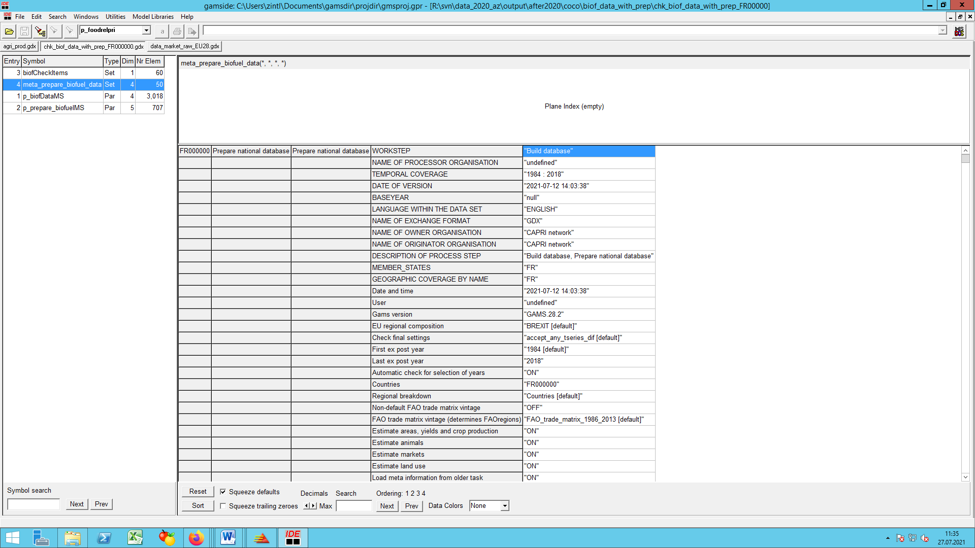
The set biofCheckItems in the same reporting .gdx file shows all biofuel items potentially filled with numbers.
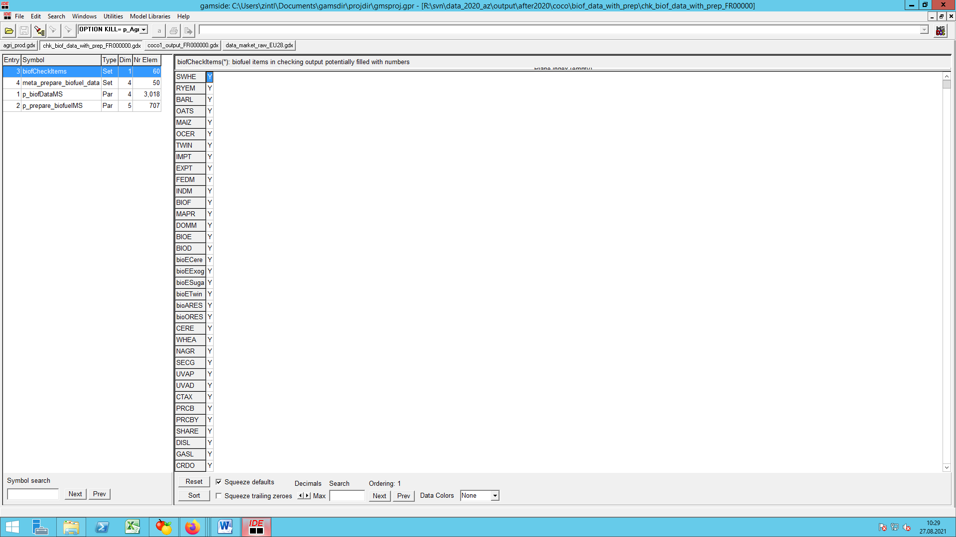
The complete list of the biofuel items in biofCheckItems includes codes which are additional to the CAPRI activity codes (see Annex on code lists above). The full code list includes the following items:
| bioECere | Ethanol processed from cereals |
| bioESuga | Ethanol processed from sugar beets |
| bioETwin | Ethanol processed from wine |
| bioEFrui | Ethanol processed from fruits |
| bioEOcro | Ethanol processed from other agricultural crops |
| bioEExog | Ethanol processed from crops not explicit in biofuel modelling (fruits, potatoes, other crops) |
| bioARES | Biofuels processed from crops residues |
| bioORES | Biofuels processed from forest residues and waste material (municipal waste, waste oil, other waste) |
| SECG | Biofuel quantities from second generation |
| MAPRagr | Ethanol production from agricultural sources |
| EloBio | Biofuel production and demand data from DG Energy project EloBio |
| DG\_Agri | Ethanol data from DGAgri website and supplementary files |
| ProdCom | Eurostat: PRODCOM ANNUAL SOLD (NACE Rev. 2.) [DS-066341] |
| EIA | Independent Statistics & Analysis, US Energy Information Administration |
| comext | Eurostat: Comext |
| Energy\_bal | Eurostat: Supply, transformation, consumption - renewable energies - annual data [nrg\_107a] |
| Energy\_dem | Eurostat: Supply, transformation, consumption - renewable energies - annual data [nrg\_102a, nrg\_1073a] |
| final | results of the calculations |
| ODOM | other domestic use (activity from biostock calculations |
| APRagr | Ethanol production from agricultural sources |
| INDt | Sum of model results for BIOF and INDM |
| BIOi, INDi, DOMi | intermediate activities to save data from model initialisation for later documentation. |
Biofuels production (levels) are calculated for biodiesel (BIOD) and bioethanol (BIOE). Input data and final initialization values before the consistency models are run are documented on the parameter p_prepare_biofuelsMS (see examples below). The results of the consistency models m_bioFitD (BIOD) and m_bioFitE (BIOE) are documented on the parameter p_biofDatatMS (see examples below).
Example 1: Bioethanol
The screenshot demonstrates the input data and final initialization values collected on parameter p_prepare_biofuelsMS. The first column of the table indicates the data source, respectively the processing status of the data. Data sources for bioethanol (BIOE) include data from EloBio, DG_Agri, ProdCom, EIA, Engergy_bal and Energy_dem. The second column of the table shows the activity.
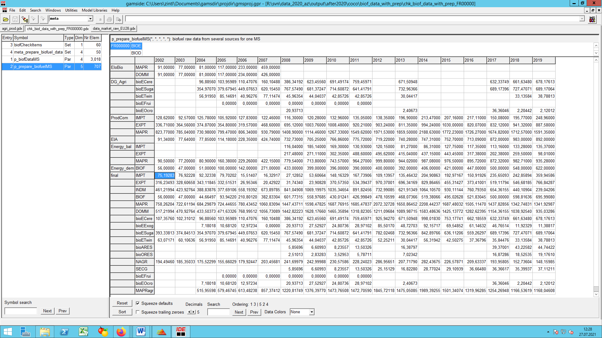
The results of the model m_bioFitE (BIOE) are documented on the parameter p_biofDatatMS.
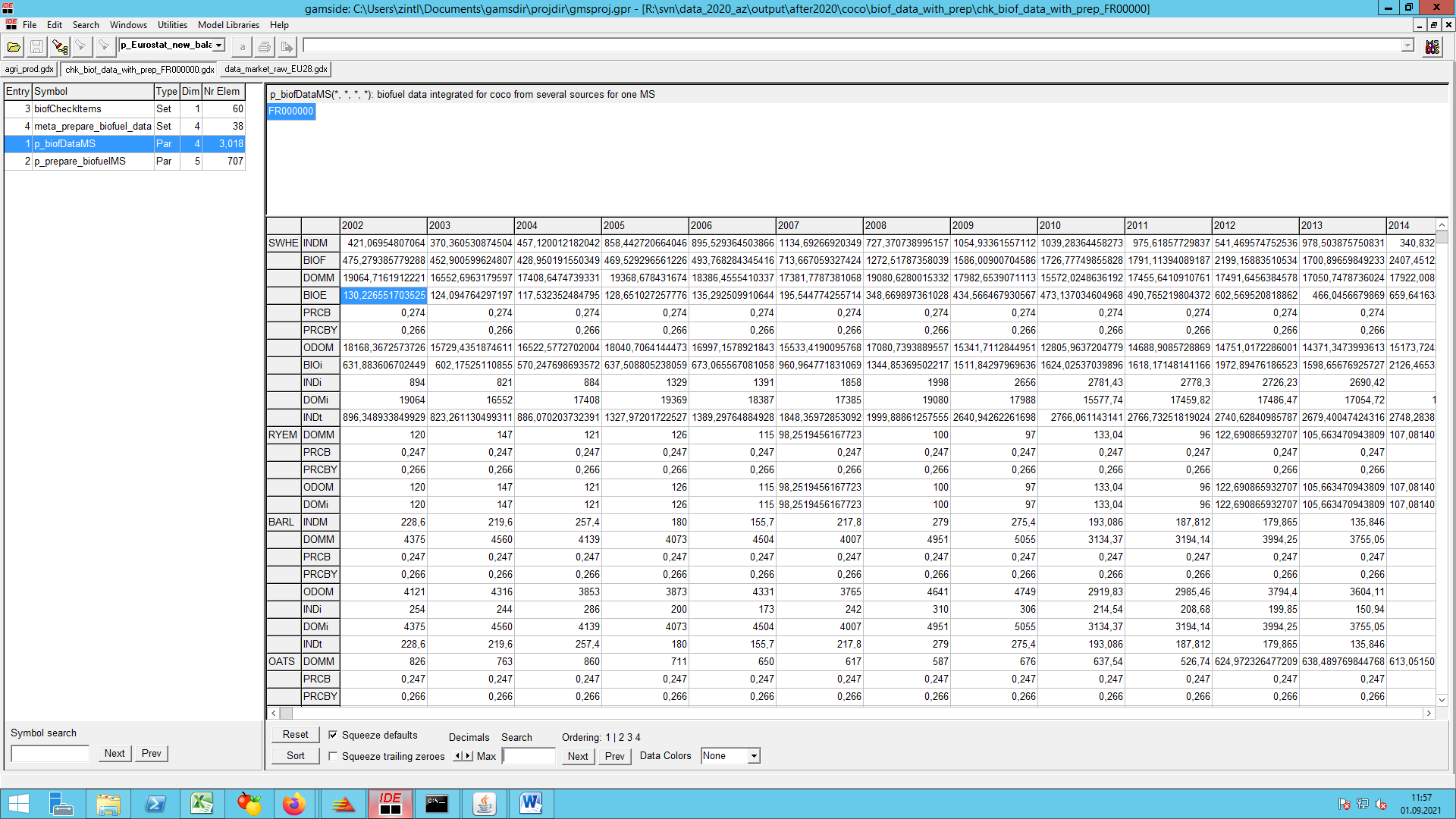
We take soft wheat (SWHE) as an example for biofuel feedstock, and walk through the initialization and consistency model results. From data input (Eurostat and FAO) we received in 2002 an industrial use of 894 1000t, saved on INDi. For production of bio-ethanol 631 1000t were initialized, saved on BIOi. The results of the breakdown by use for bio-ethanol and others industrial use, are saved on BIOF and INDM. BIOE shows the yield of soft wheat for bio-ethanol.
Example 2: Biodiesel
The first dimension of the reporting parameter p_prepare_biofuels shows the data source (processing status). The second dimension of the parameter shows the activity.
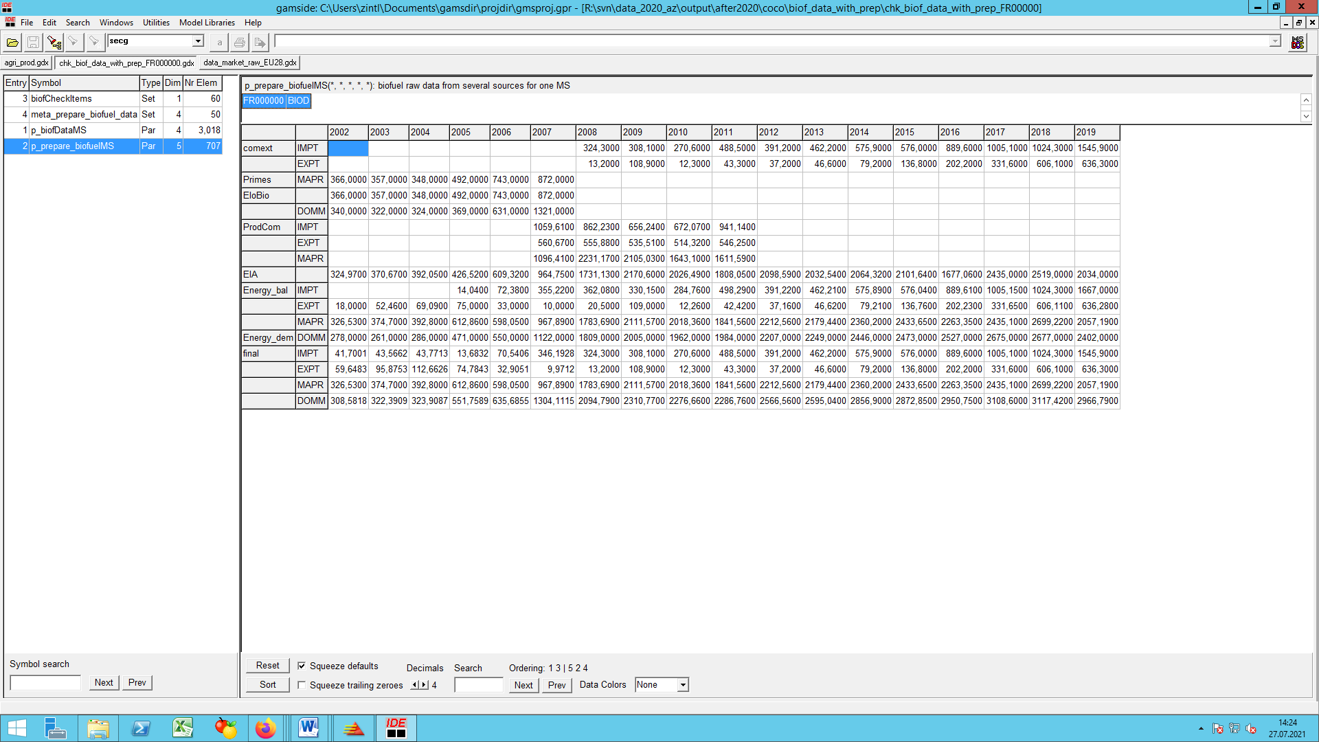
For Bio-diesels, PRIMES model results are used as an additional data source.
| Data source code | Data source description |
|---|---|
| Primes | PRIMES MODEL, EC3MLAB of ICCS, National University of Athens |
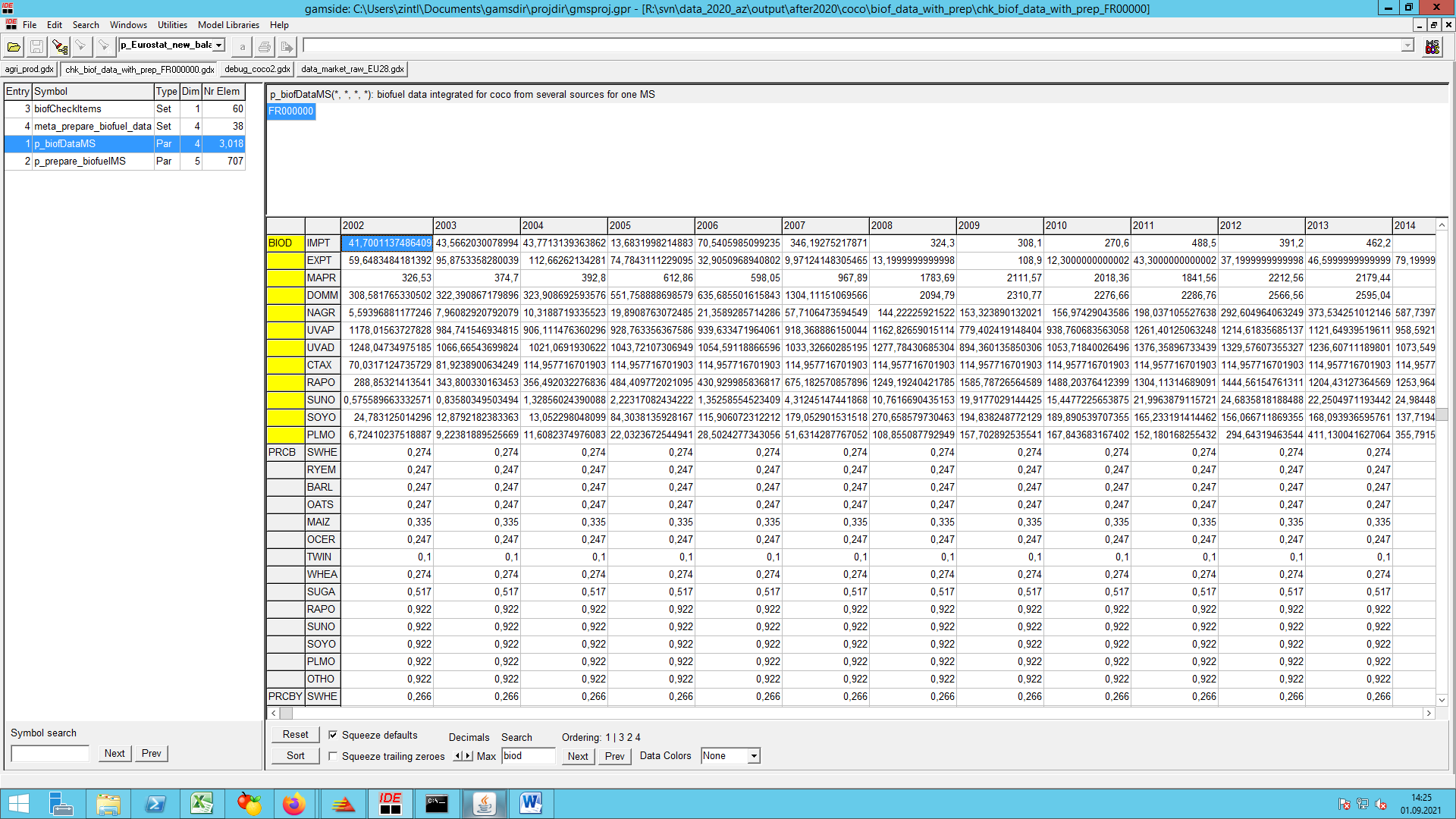
The parameter p_biofDataMS reports on production (MAPR), trade (import:IMPT, export:EXPT), production from non-agricultural sources (NAGR), prices (UVAD, UVAP) and consumer taxes (CTAX). The distribiutio of total biodiesel processing to the feedstock is also reported, for rapeseed oil (RAPO), sunflower oil (SUNO), soya oil (SOYO) and palm oil (PLMO).
Annex: Testing procedure and checking intermediate steps in COCO (dairy)
The following three examples show how to use the intermediate reporting files to trace the data preparation steps. Screenshots demonstrate the arrangement of the reporting parameters by using the CAPRI Graphical User Interface. COCO automatically produces the reporting files in the folder results/coco/res_estima/
Example 1: Production of cow (COMI) and sheep (SGMI) milk
In order to document the procedure of data consolidation and rebooking, we look at the reporting file for France “chk_estima_FR000.gdx”.
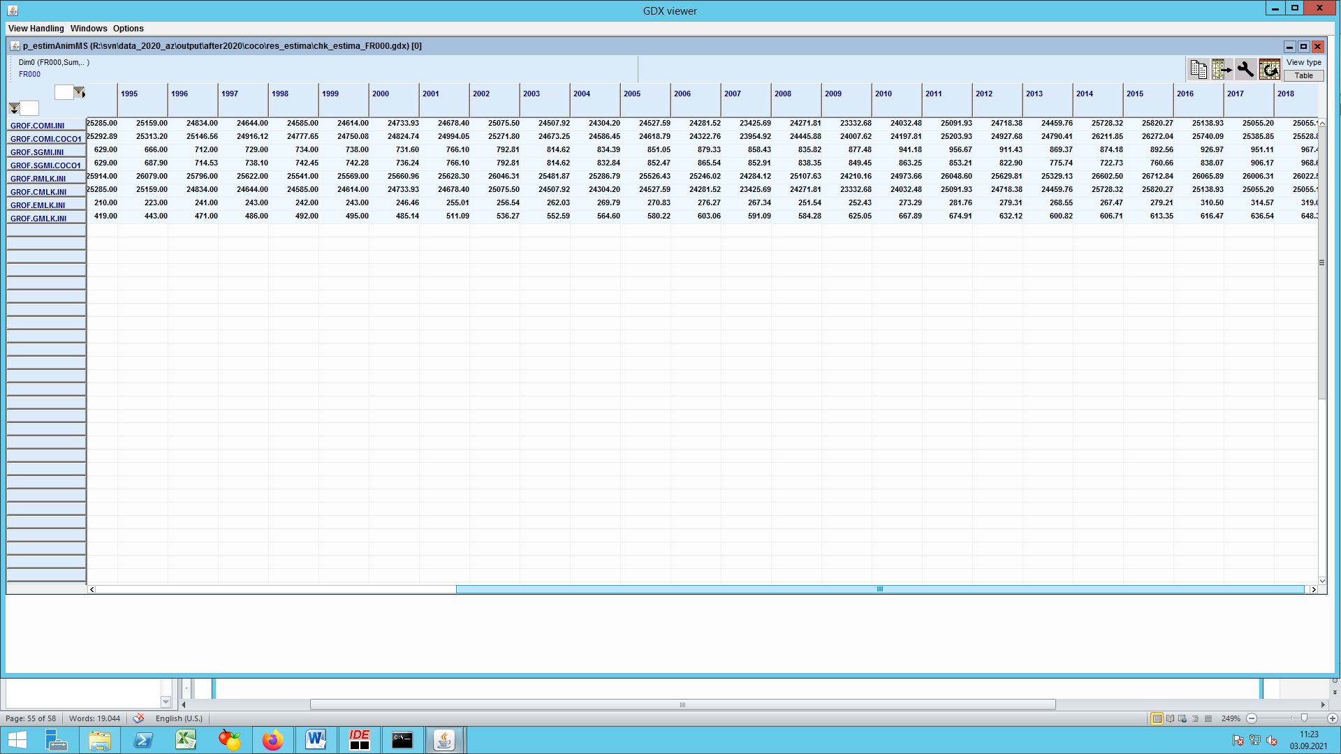
The codes in the rows show the activity code, the product code and its status. For activity codes see Annex 1: Code list.
Status codes:
- INI: initial value
- COCO1: estimation value
The initialization of the production of COMI and SGMI is done in the module coco1_milk.gms (see section 3.1.3). Additional remarks to better understand the example:
- COMI: Milk from cows (CMLK) and buffaloes (BMLK) is added up.
- SGMI: Milk from ewes (EMLK) and goats (GMLK) is added up.
- If data on cow or sheep and goat milk is not available separately, but total milk production (RMLK) is available, then production of COMI is set equal to total milk production.
- Only COMI and SGMI are included in the estimation in coco1_estima.gms
- The production of RMLK and its components CMLK, BMLK, EMLK and GMLK are only copied from raw data tables into this check parameter for documentation purposes.
Example 2: data consolidation for cow milk
The procedure of data consolidation and rebooking of all activities for the CAPRI product “COMI” (cow milk) is shown in the following screenshot (only part of the reporting parameter p_estimAnimMS is shown, but the full scope of the table is visible in the GUI).

The codes in the rows show the activity code and its status. For activity codes see Annex 1: Code list. Additional codes for status include the following.
| Status code | Status code description |
|---|---|
| StdeData | Final (small) Stde (standard deviation) attached to priors from raw data |
| StdeScale | Final (large) Stde attached to priors from trends but not from raw data |
| Upplim | Soft upper limits triggering extra penalties if violated |
| Lowlim | Soft lower limits triggering extra penalties if violated |
| Supps | Prior value = support: comes from raw data or trends plus HP filter |
| Err2rev | Original error term from preest: to steer speed of bound opening |
Under activity dairy cows (DCOW) the following items are reported: yield, total production (GROF), feed use (FEDM) and losses on market (LOSM). Eurostat’s National Accounts of Agriculture (EAA) only supply data for the aggregate milk (MILK). The equation e_EAAMLK in the consolidation model AnimNSSQ ensures the consistency of EAA values for MILK, as they are split up between cow milk (COMI) and sheep and goat milk (SGMI).
e_EAAMLK("%MS%000",T)
     $ (p_NobsP("%MS%000","EAAP","MILK") AND ESTR("MILK") and
        (p_NobsP("%MS%000","EAAP","COMI") or p_NobsP("%MS%000","EAAP","SGMI"))) ..
*
        v_EstimY("%MS%000","EAAP","MILK",T) =E=
                             v_EstimY("%MS%000","EAAP","COMI",T) $ p_NobsP("%MS%000","EAAP","COMI")
                           + v_EstimY("%MS%000","EAAP","SGMI",T) $ p_NobsP("%MS%000","EAAP","SGMI") ;
Finally. the producer prices (UVAP) are calculated directly from the monetary EEA values and production. The following picture shows the data processing steps (states) for the EAA values for milk.
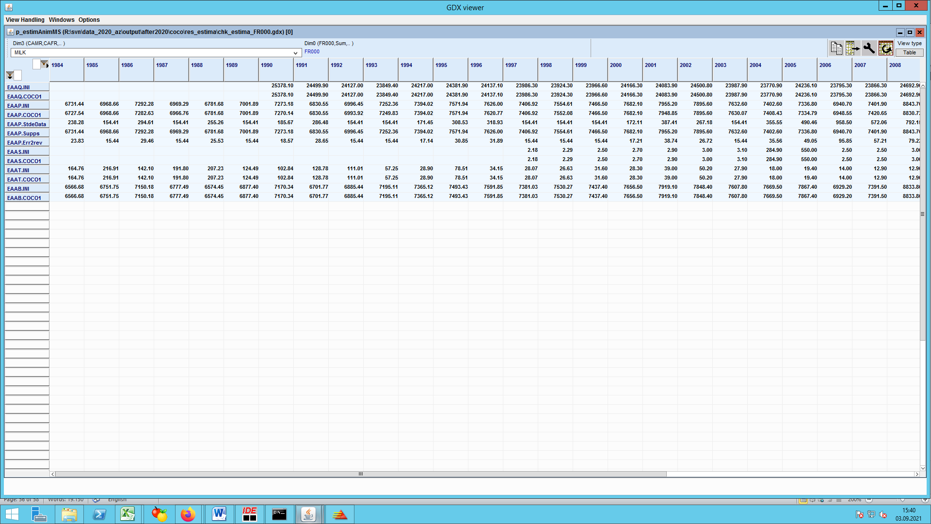
From the example for COMI above you can also understand the influence of the standard deviation from raw data (e.g. FEDM.StdeData), and standard deviation from trends (e.g. FEDM.StdeScale) Standard deviations are calculated both for raw data and the trends. For years where FEDM.StdeData is given, the results are very close to the prior values FEDM.Supps, whereas they are deviating sizeably for years where only FEDM.StdeScale is available.
The first initialisation of StdeData and StdeScale is done in module coco1_preest.gms, which is a pre-step for the data consolidation models (crops, animals, market balances), using a Hodrick-Prescott filter to smooth the combination of given values and trend line. Both standard deviations enter the objective function (see chapter 3.1.4).
Example 3: data consolidation for cow dairy cow activity (DCOW)
The procedure of data consolidation and booking intermediate data processing results for the dairy cow activity (DCOW) is demonstrated in the following screenshot.
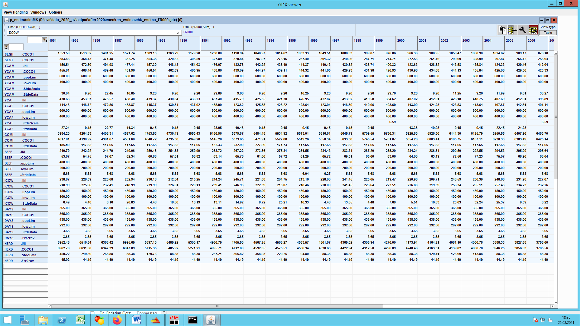
The rows of the table show the product item code for the production activity DCOW, and the data processing steps (status). The first two lines show the coco1 results for slaughtering. The items starting with Y and I stand for the output and input of calves. The initialization, the estimation steps and the final results are all documented on the reporting parameter p_estimAnimMS. Items COMI and BEEF show the yields for cow milk and beef. Item DAYS is the process length, initialized by 365 days (equals one year). Finally, the item HERD models the herd size of dairy cows.
The Regionalised Data Base (CAPREG)
Data requirements and sources at the regional level
CAPRI aims at building up a Policy Information System of the EU’s agricultural sector, regionalised at NUTS 2 level or farm types inside NUTS 2 regions with an emphasis on the impact of the CAP. The core of the system consists of a regionalized or farm type agricultural sector model using an activity based non-linear programming approach. One feature of such a highly disaggregated, activity based agricultural sector model is the detailed information resulting from ex ante simulations of policy scenarios concerning the output and input of specific agricultural production activities and their relationships. This information is also a pre condition to judge possible impacts of agricultural production on the environment. However, these systems require as well this kind of information (data) ex-post, at least partially. It is especially necessary to define for each region in the model, at least for the basis year, the matrix of I/O-coefficients for the different production activities together with prices for these outputs and inputs. Moreover, for calibration and validation purposes information concerning land use and livestock numbers is necessary.
Already from the beginning of the development of the CAPRI model, the regional agricultural statistics (EUROSTAT table group reg_agr) was judged as the only harmonized data source available on regionalized agricultural data in the EU. Other regional Eurostat data are suplementing the regional agricultural statistics such that we are currently using the following:
- Land use from regional landuse statistics [agr_r_landuse, discontinued table]
- Land cover from LUCAS [lan_lcv_ovw, currently only used in COCO1]
- Crop production - harvested areas, production and yields [table agr_r_crops]
- Animal production - livestock numbers [table agr_r_animal]
- Milk production [agr_r_milkpr]
- Agricultural accounts on regional level [table agr_r_accts]
- Structure of agricultural holdings including labour force [ef_ls_ovlsureg, ef_olslsureg, ef_oluaareg, ef_oluaareg, ef_r_nuts]
Although the content of the regional datasets has remained in time, the naming and classification within EUROSTAT is undergoing continuous modifications. Tables considered of low interest are discontinued (and may be still used in CAPRI some time after this point, such as table agr_r_landuse). And new topics are covered providing useful data in some areas, for example from agri-environmental indicators (table reg_aei):
- Estimated soil erosion by water, by NUTS 3 regions (aei_pr_soiler)
- Manure storage facilities by NUTS 3 regions (aei_fm_ms)
The following table shows the availability of the different regional tables as they have been used in the current database (with series completed up to 2014). However, the current coverage concerning time and sub-regions differs dramatically between the tables and within the tables between the Member States. A second problem consists in the relatively high aggregation level especially in the field of crop production. Hence, additional sources, assumptions and econometric procedures must be applied to close data gaps and to break down aggregated data.
Table 6 Availability of regional datain current database after 1983
| Table | Official availability |
|---|---|
| Land use | from 1974 yearly |
| Crop production (harvested areas, production and yields) | from 1975 yearly |
| Animal production (livestock numbers) | from 1977 yearly |
| Agricultural accounts on regional level | from 1980 yearly |
| Structure of agricultural holdings and labour force | 2000, 2003, 2005, 2007, 2010, 2013 |
Source: capri/dat/capreg/regio_data_all.gdx
Methodology applied in the regional data consolidation
In the last major update of 2015 the original data had been first stored in the TSV format designed by EUROSTAT:
- Unordered List ItemIn a first step, these files had been converted by an excel macro into csv format and an overall set with all items including their long text has been created to prepare further processing.
- In a second step these alredy GAMS readable files are stored in GDX format in folder “dat/capreg” and under version control. Meta data are added in the process as well.
The results of these two steps is a single large tables, which comprise time series of all data retrieved from Eurostat for all tables: land use, crop production, animal populations, cow’s milk collection and agricultural accounts.
The starting point of the methodological approach is the decision to use the consistent and complete national data base (COCO) as a frame or reference point for any regionalization. In other words, any aggregation of the main data items (areas, herd sizes, gross production and intermediate use, unit value prices and EAA-positions) of the regionalized data over regions must match the national values. This is the general rule with some exceptions.
Given that starting position, the following approaches are generally applied:
- Unordered List ItemData as loaded from the regional statistics are subject to some manual consistency checks (in gams/capreg/check_and_cor_regio.gms) as well as checks for regional consistency. The latter is mainly true for animal herd sizes where we have data at the same or even more disaggregated level as found in COCO.
- Gaps in regional data are completed and data only given at a higher aggregation level as required in CAPRI are broken down by using existing national information.
- Fall back and other rules for assignments are structurally and (often) numerically identical for all regional units and groups of activities and inputs/outputs.
- Econometric analysis or additional data sources are used to close gaps.
All the approaches described in the following sub sections are only thought as a first crude estimate. Wherever additional data sources are available, their content should be checked and is often used to overcome the list of these ‘easy to use’ estimates presented in here. Examples are (some) data for Norway, Sweden or Luxembourg that have been collected from national sources. The procedures described in here can be thought as a ‘safety net’ to ensure that regionalized data are technically available but not as an adequate substitute for collecting these data from additional sources.
Prices
The agricultural domain of REGIO does not cover regionalized prices. For simplicity, the regional prices are therefore assumed to be identical to sectoral ones13):
\begin{equation} UVAG_r=UVAG_s \end{equation}
Young animal prices are a special case since they are not included in the COCO data base (the current methodology of the EAA does not value intermediate use of animals) but are necessary to calculate income indicators for intermediate activities (e.g. raising calves). Only exported or imported live animals are implicitly accounted for by valuing the connected meat imports and exports.
Young animals are valued based on the ‘meat value’ and assumed relationships between live and carcass weights. Male calves (ICAM, YCAM) are assumed to have a final weight of 55 kg, of which 60 % are valued at veal prices. Female calves (ICAF, YCAF) are assumed to have a final weight of 60 kg, of which 60 % are valued at veal prices. Young heifers (IHEI, YHEI) are assumed to have a final weight of 300 kg, of which 54 % are valued at beef. Young bulls (IBUL, YBUL) are assumed to have a final weight of 335 kg, of which 54 % are valued at beef. Young cows (ICOW, YCOW) are assumed to have a final weight of 575 kg, of which 54 % are valued at beef. For piglets (IPIG, YPIG), price notations were regressed on pig meat prices and are assumed to have a final weight of 20 kg of which 78 % are valued at pig meat prices. Lambs (ILAM, YLAM) are assumed to weight 4 kg and are valued at 80 % of sheep and goat meat prices. Chicken (ICHI, YCHI) are assumed to weight 0.1 kg and are valued at 80 % of poultry prices.
Another special case are sugar beet prices. They are still determined in a program (‘sugar/price_est.gms’) inherited from the 2003 EuroCARE sugar study (Henrichsmeyer et al. 2003). It determines sugar beet prices according to the sugar prices, levies and partial survey results in the 90ies. The estimation results are subsequently used to determine the beet price differentiation also in subsequent years. It is noteworthy that the same program is applied in CAPREG (via quotasprices.gms) and in CAPMOD (via data_prep.gms) to determine base year beet prices.
Activity Levels
In cases where data on regional activity levels are missing, a linear trend line is estimated for regional and Member State time series in the definition of the regional database. The gap is then filled with a weighted average between the trend line – using a weight of R² - and a weighted average of the available observations around the gap, using a weight of 1-R². The specific formulation has the following properties. In cases of a strong trend in a time series, the back-casted and forecasted numbers will be dominated by the trend as the weight of R² will be high. With decreasing R², the estimated values will be pulled towards known values.
Apart from gap filling another problem is that in annual cropland statistics at the regional level only cover a few crop activities (cereals with wheat, barley, grain maize, rice; potatoes, sugar beet, oil seeds with rape and sunflower; tobacco, fodder maize; grassland, permanent crops with vineyards and olive plantations). The COCO data base, however, covers some 30 different crop activities. In order to break these aggregates down to COCO definitions, the national shares of the aggregate are used.
As an example, this approach is explained for cereals. Data on the production activities WHEA (wheat = SWHE+DWHE), BARL (barley), MAIZ (grain maize) and PARI (paddy rice) as found in COCO match directly the level of disaggregation in the regional data. Therefore, the mapped regionalized data are directly set equal to the corresponding values in the regional “raw” data. The difference between the sum of these 4 activities and the aggregate data on cereals in the regional raw data must be equal to the sum of the remaining activities in cereals as shown in COCO, namely RYE (rye and meslin), OATS (oats) and OCER (other cereals). As long as no other regional information is available, this difference from the regional raw data is hence broken down applying national shares.
The approach is shown for OATS in the following equations, where the suffix r stands for regional data:
\begin{align} \begin{split} LEVL_{OATS,r} &= (CEREAL_r\\ &\quad -WHEAT_r-BARLEY_r-MAIZEGR_r-RICE_r)\cdot\\ &\quad\frac{LEVL_{OATS,COCO}}{(LEVL_{OATS,COCO}+LEVL_{RYE,COCO}+LEVL_{OCER,COCO})} \end{split} \end{align}
Similar equations are used to break down other aggregates and residual areas in the regional data 14). The Farm Structure Survey (FSS) provides crop areas for a larger number of crops but this survey is usually conducted only every three years. Data from FSS, when available, is also used to aproximate crop areas at regional level.
One important advantage of the approach is the fact that the resulting areas are automatically consistent to the national data if the ingoing information from REGIO was consistent to national level. Fortunately, the regional information on herd sizes covers most of the data needed to give nice proxies for all animal activities in COCO definition. The regional data break down for herd sizes is often more detailed than COCO at least for the important sectors. Regional estimates for the activity levels are therefore the result of an aggregation approach, in opposite to crop production.
In order to generate good starting points for the following steps of data processing and to avoid systematic deviations between regional and national levels in the following consistency steps, all regional level in REGIO are first scaled with the relation between the (national) results in COCO and the regional results when aggregated to the national level (key file is gams/capreg/map_from_regio.gms).
Besides technological plausibility and a good match with existing regional statistics, the regionalized data for the CAPRI model must be also consistent to the national level. The minimum requirement for this consistency includes activity levels and gross production. The “initialisation” of the regional database has been undertaken already to meet this requirement as good as possble but cannot guarantee it. Consistency for activity levels is therefore based on Highest Posterior Density Estimator which ensures (in gams/capreg/cons_levls.gms):
- Adding up of activity levels from lower regional level (NUTS II, NUTS I) to higher ones (NUTS I, NUTS 0)
- Adding up of crop areas to UAA at regional level.
The objective function minimizes in case of animal herds simple squared relative deviations from the herds. In case of crops, a 25% weight for absolute squared difference of the crop shares on UAA plus 75% deviation of relative squared differences is introduced. In the crop sector consistency is also imposed to regional transition matrices for 6 UNFCCC land use categories relevant for carbon accounting (forest land, cropland, grassland, settlements, wetlands, residual land) which are initialised from the national transition matrix estimated in the COCO1 module.
A specific problem is the fact that land use statistics do not report a break down of idling land into obligatory set aside, voluntary set aside and fallow land15). Equally, the share of oilseeds grown as energy crops on set aside needs to be determined. An Highest Posterior density estimator is used (in gams/capreg/cal_seta.gms) to ‘distribute’ the national information on the different types of idling land to regional level, with the following restrictions:
- Obligatory set-aside areas must be equal to the set-aside obligations derived from areas and set-aside rates for Grandes Cultures (which may differ at regional level according to the share of small producers). For these crops, activity levels are partially endogenous in the estimation in order to allow a split up of oilseeds into those grown under the set-aside obligations and those grown as non-fo-od crops on set-aside.
- Obligatory and voluntary set-aside cannot exceed certain shares of crops subjects to set-aside (at least before Agenda 2000 policy)
- Fallow land must equalise the sum of obligatory set-aside, voluntary set-aside and other idling land.
- Total utilisable area must stay constant.
In some cases, areas reported as fallow land are smaller than set-aside obligations. In these cases, parts of grassland areas and ‘other crops’ are allowed to be reduced.
Production and yields
The proceedure for gross output (GROF) is similar to the one for activity levels, as correction factors are applied to line up regional yields with given national production:
\begin{align} \begin{split} CORR_{GROF,o} &= \sum_{j,r}{Levl_{j,r}O_{j,r}}/GROF_{o,n}\\ O_{j,r}^*&=O_{j,r} \cdot CORR_{GROF,o} \end{split} \end{align}
In case of missing statistical information for regional yields, national yields are used. A special rule is used for fodder maize yields, where regional yields are derived from national fodder maize yields, and the relation between regional and national average cereal yields.
For grassland and fodder from arable land, missing yields are derived from national ones using the relation between regional and national stocking densities of ruminants, in combination with assumed share of concentrates in terms of a weighted sum of energy and protein per ruminant activity in CAPRI. Those shares are then scaled with a uniform factor to exhaust on average the available energy and protein from concentrates at the national level. Accordingly, higher fodder yields are expected where ruminant stocking densities are high, acknowledging differences in concentrate shares. If e.g. the stocking densities solely stem from sheep and goat, the assumed impacts on yields is higher. In order to avoid unrealistic low or high yields, those are bounded to a 25%-400% range compared to the regional aggregate.
The input allocation in any given year should not be linked to realised, but to expected yields. Expected yields are constructed using the following modified Hodrick-Prescott filter:
\begin{equation} \text{min} \quad hp=1000 \sum_{1<t<T-1}({y_{t+1}^*-y_{t-1}^*})^2 + \sum_{t}({y_t^*-y_t})^2 \end{equation}
where y covers all output coefficients in the data base. The Hodrick-Prescott filter is applied both at the national and regional level after any gaps in the time series had been closed.
Final steps of regional data completion
The regional database modules also cover some aspects which are discussed in other parts of this documentation.
- For policy data at the regional level (mostly premium related data) see Section Policy data. These policy related assignments require a good part of the CAPREG module
- For the fertiliser and feed allocations and environmental indicators, also important elements of the regional database, see the next Section Input Allocation
- Towards the end of the regional data base consolidation supply side PMP parameters are calibrated as a final test of consistency and sometimes to serve as starting values for the subsequent baseline calibration (in gams/capreg/pmp.gms)
Build and compare time series of GHG inventories
The regionalised data base module CAPREG runs in two steps:
- The first steps prepares regional time series covering activities, production, land use and the fertiliser allocation
- The second step involves more time consuming processing steps which are therefore only executed for the selected base year: feed allocation, computation of GHG results, and the final calibration test
To assess the reliability of the CAPRI database in terms of GHG results against official UNFCCC notifications, results from the first step (time series) were insufficient, as the GHG accounting also requires information on the feed allocation. This problem was addressed within the scope of the IDEAg (Improving the quantification of GHG emissions and flows of reactive nitrogen) project16), where an option has been introduced to allow for a consistent accounting of GHG emissions over time. This is able to combine input information from CAPREG time series runs as well as (short run, nowcasting-style) CAPMOD simulation results. Furthermore, an R-based tool was introduced to the CAPRI GUI that maps GHG emissions data from CAPRI to the GHG emission balances contained in the National Inventory Reports (NIRs) that are submitted annually by countries in compliance with UNFCCC GHG reporting obligations.
Input Allocation
The term input allocation describes how aggregate input demand (e.g. total anorganic N fertiliser use in Denmark) is ‘distributed’ to production activities. The resulting activity specific data are called input coefficients. They may either be measured in value (€/ha) or physical terms (kg/ha). The CAPRI data base uses physical terms and, where not available, input coefficient measured in constant prices.
Micro-economic theory of a profit maximising producer requires revenue exhaustion, i.e. marginal revenues must be equal to marginal costs simultaneously for all realised activities. The marginal physical input demand multiplied with the input price exhausts marginal revenues, leading to zero marginal profits. Marginal input demands per activity can only be used to define aggregate input demand if they are equal to average input demands. The latter is the case for the Leontief production function.
The advantage of assuming a Leontief technology in agricultural production analysis is the fact that an explicit link between production activities and total physical input use is introduced (e.g. environmental indicators can be linked directly to individual activities or activity specific income indicators, since gross margins can be calculated). The disadvantage is the rather rigid technology assumption. We would for example expect that increasing a crop share in a region will change the average soil quality the crop uses, which in turn should change yields and nutrient requirements. It should hence be understood that the Leontief assumption is an abstraction and simplification of the ‘real’ agricultural technology in a region. The assumption is somewhat relaxed in CAPRI as two ‘production intensities’ are introduced.
Input coefficients for different inputs are constructed in different ways which will be discussed in more detail in the following sections:
- For nitrate, phosphate and potash, nutrient balances are constructed so to take into account crop and manure nutrient content and observed fertiliser use, combined with gaseous losses. These balances ex post determine the effective input coefficients and regional availability of manure and overfertilisation parameters.
- For feed, the input calculation is rooted in a mix of engineering knowledge (requirement functions for animal activities, nutrient content of feeding stuff, recommendations on feed mix), observed data ex post (total national feed use, national feed costs), combined within a Highest Posterior Density (HPD) estimation framework.
- For the remaining inputs, estimation results from a FADN sample in the context of the CAPSTRAT project (2000-03) are combined with current aggregate national input demand reported in the EAA and standard gross margin estimations, again using a HPD estimation framework.
Input allocation excluding young animals, fertiliser and feed
There is a long history of allocating inputs to production activities in agricultural sector analysis, dating back to the days where I/O models and aggregate farm LPs where the only quantitative instruments available. In these models, the input coefficients represented a Leontief technology, which was put to work in the quantitative tools as well. However, input coefficients per activity do not necessary imply a Leontief technology. The allocated input demands can be seen as marginal ones (which are identical to average ones in the Leontief case) and are then compatible with flexible technologies as well.
Input coefficients can be put to work in a number of interesting fields. First of all, activity specific income indicators may be derived, which may facilitate analyzing results and may be used in turn to define sectoral income. Similarly, important environmental indicators are linked to input use and can hence be linked to activities as well with the help of input coefficients.
Given the importance or the input allocation, the CAP STRAT project (2000-2003) comprised an own work package to estimate input coefficients. On a first step, input coefficients were estimated using standard econometrics from single farm record as found in FADN. Additionally, tests for a more complex estimation framework building upon entropy techniques and integrating restrictions derived from cost minimization were run in parallel. The need to accommodate the estimation results with data from the EAA in order to ensure mutual compatibility between income indicators and input demand per activity and region on the one hand, and sectoral income indicators as well as sectoral input use on the other, requires deviating from the estimated mean of the coefficients estimated from single farm records. Further on, in some cases estimates revealed zero or negative input coefficients, which cannot be taken over. Accordingly, it was decided to set up a second stage estimation framework building upon the unrestricted estimates from FADN. The framework can be applied to years where no FADN data are available, and thus ensures that the results will be continuously used for the years ahead, before an update of the labor-intensive estimations is again necessary and feasible.
As a result of the unrestricted estimation based on FADN 17)a matrix of input coefficients for 11 input categories (Total Inputs, Crop Only Inputs, Animal Only Inputs, Seeds, Plant Protection, Fertilizer, Other Crop Inputs, Purchased and Non-Purchased Feeds and Other Animal Only Inputs) and their estimated standard errors is available. Some of those coefficients are related to the output of a certain activity (e.g. how much money is spend on a certain input to produce one unit of a product), some of them are related to the acreage of on activity (input costs per activity level).
All of the econometric coefficients were required to be transformed into an ‘activity level’ form, due to the fact that this is the definition used in the CAPRI model. Before this could be done, it seemed necessary to fill up the matrix of estimated coefficients because some estimates were missing and others were negative. In order to this we constructed a number of coefficients that were weighted averages among certain groups. These mean coefficients were the following.
- Mean coefficients of activity groups. Each activity was allocated to a certain group (e.g. soft wheat belonged to cereals). For each group we built weighted averages among the positive estimates within a group using the estimated t statistics as weights. This coefficient only existed if there was at least one positive estimate inside that group and was then used to replace the gaps inside the coefficient matrix. If that mean coefficient was not available, due to no positive estimate inside a group at all, the next type of mean coefficients became relevant:
- Mean coefficients for an activity among European regions. This second type of mean coefficients calculates weighted averages among three types of regional clusters. These clusters are Northern European States, Southern European states and all European regions. Again, the estimated t statistics were used as aggregation weights. Unfortunately, this type of averages did not fill all gaps in the coefficient matrix as there were some activities that had no positive estimate over the entire EU. For those the third type of mean coefficients was calculated.
- Mean coefficients for activity groups among regional clusters. Here we calculated for the three regional clusters the averages of the first type of mean coefficients. As even the latter are synthetic, we gave each mean of them the same weight. Fortunately there was only a small probability that this coefficient did not exist for one of the groups as this was only the case if no coefficient inside a group over the entire EU had a positive estimate, which was not the case.
Following these rules we finally got a matrix of estimated and synthetic calculated input coefficients for both, the ‘per activity level’ and the ‘per production’ unit definition18). For the synthetic one there was no estimated standard error available but we wanted to use those later on. So we assumed them –to reflect that these coefficients have only weak foundation– to have a t statistic of 0.5.
The ‘per level’ definition was only taken over if the coefficient was really estimated or if no per production unit definition did exist. To transfer the latter into per activity level definition, we multiplied them with the average yield (1985 2001) of the respective activity. The resulting coefficients and their standard errors were then used a HPD approach as a first set of priors19).
Missing econometric estimates and compatibility with EAA figures were not the only reasons that made a reconciliation of estimated inputs coefficients necessary. Moreover, the economic sense of the estimates could not be guaranteed and the definition of inputs in the estimation differed from the one used in CAPRI. Therefore we decided to include further prior information on input coefficients in agriculture. The second set of priors in the input reconciliation was therefore based on data from the EAA. Total costs of a certain input within an activity in a European Member State was calculated by multiplying the total expenditures on that input with the proportion of the total expected revenue of that activity to that of all activities using the input. Total expected revenue in this case was the production value (including market value and premiums) of the respective activity. If this resulted in a certain coefficient being calculated as zero due to missing data, then this coefficient would be replaced by one from a similar activity e.g. a zero coefficient for ‘MAIF’ would be replaced by the coefficient for ‘GRAS’
This kind of prior information tries to give the results a kind of economic sense. For the same reason the third type of priors was created based on standard gross margins for agricultural activities received from EUROSTAT. Those existed for nearly all activities. The set from 1994 was used, since this was the most complete available. Relative rather than absolute differences were important, given the requirement to conform to EAA values20).
Given the three types of prior information explained above –estimated input coefficients, data from EAA and standard gross margins , a HPD estimator has been used to reconcile the prior information on input coefficients. Accounting constraints ensure (see in “dist_input.gms”) first that gross margins for an activity is the difference between expected revenue per activity level of that activity and the sum over all inputs used in that activity and second that the sum over all activities of their activity levels multiplied with an input gives the total expenditures on that input given by the EAA. The estimation is carried out in GAMS within and run for each year in the database. Some bounds are further set to avoid estimates running into implausible ranges.
The Highest Posterior Density estimation yields monetary input coefficients for the fertiliser types (Nitrate, Phosphate, Potassium), seeds, plant protection, feeds, pharmaceutical inputs, repairs, agricultural service input, energy and other inputs. While some of these can be directly used in the CAPRI model, we need special treatments for others –e.g. fertilisers, because they are used in physical units inside the model, and feeds, since they are much more disaggregated.
Input allocation for young animals and the herd flow model
Figure below shows the different cattle activities and the related young animal products used in the model. Milk cows (DCOL, DCOH) and suckler cows (SCOW) produce male and female calves (YCAM, YCAF). The relation between male and female calves is estimated ex post in the COCO framework. These calves are assumed to weigh 50 kg at birth (see gams/feed/feed_decl.gms) and to be born on the 1st of January. They enter immediately the raising processes for male and female calves (CAMR, CAFR) which produce young heifers (YHEI, 300 kg live weight) and young bulls (YBUL, 335 kg). The raising processing are assumed to take one year, so that calves born in t enter the processes for male adult fattening (BULL, BULH), heifers fattening (HEIL, HEIH) or heifers raising (HEIR) on the 1st January of the next year t+1. The heifers raising process produces then the young cows which can be used for replacement or herd size increasing on the first of January of t+2. The table below the diagram shows a numerical example (for DK, 1999-2001) for these relationships.
Figure 5: The cattle chain

Accordingly, each raising and fattening process takes exactly one young animal on the input side. The raising processes produce exactly one animal on the output side which is one year older. The output of calves per cow, piglets per sow, lambs per mother sheep or mother goat is derived ex post, e.g. simultaneously from the number of cows in t-1, the number of slaughtered bulls and heifers and replaced in t+1 which determine the level of the raising processes in t and number of slaughtered calves in t. The herd flow models for pig, sheep and goat and poultry are similar, but less complex, as all interactions happen in the same year, and no specific raising processes are introduced.
Table 7: Example for the relation inside the cattle chain (Denmark, 1999-2001)
| 1999 | 2000 | 2001 | ||
|---|---|---|---|---|
| Male calves used in t and born in t | ||||
| DCOWLEVL | Number of dairy cows | 667,03 | 654,08 | 631,92 |
| DCOWYCAM | Number of male calves born per 1000 dairy cows | 420,72 | 438,62 | 438,26 |
| Number of males calves born from dairy cows | 280,63 | 286,89 | 276,95 | |
| SCOWLEVL | Number of suckler cows | 127,36 | 126,91 | 124,85 |
| SCOWYCAM | Number of male calves born per 1000 suckler cows | 420,72 | 411,83 | 401,61 |
| Number of male calves born from suckler cows | 53,58 | 52,27 | 50,14 | |
| Number of all male calves born | 334,22 | 339,16 | 327,09 | |
| GROFYCAM | Number of male calves produced | 334,21 | 339,16 | 327,09 |
| CAMFLEVL | Number of male calves fattened | 81,32 | 72,57 | 49,18 |
| CAMRLEVL | Activity level of the male calves raising process | 252,89 | 266,59 | 277,91 |
| Sum of processes using male calves | 334,21 | 339,16 | 327,09 | |
| GROFYCAM | Number of male calves used | 334,21 | 339,16 | 327,09 |
| Female calves used in t and born in t | ||||
| DCOWLEVL | Number of dairy cows | 667,03 | 654,08 | 631,92 |
| DCOWYCAF | Number of female calves born per 1000 dairy cows | 404,15 | 421,58 | 412,86 |
| Number of female calves born from dairy cows | 269,58 | 275,75 | 260,89 | |
| SCOWLEVL | Number of suckler cows | 127,36 | 126,91 | 124,85 |
| SCOWYCAF | Number of male calves born per 1000 suckler cows | 404,15 | 398,04 | 387,21 |
| Number of female calves born from suckler cows | 51,47 | 50,52 | 48,34 | |
| Number of all female calves born | 321,05 | 326,26 | 309,24 | |
| GROFYCAF | Number of female calves produced | 321,05 | 326,27 | 309,24 |
| CAFFLEVL | Number of female calves fattened | 26,64 | 28,74 | 18,39 |
| CAFRLEVL | Activity level of the female calves raising process | 294,41 | 297,53 | 290,85 |
| Female calves used in t and born in t | 321,05 | 326,27 | 309,24 | |
| GROFYCAF | Number of female calves used | 321,05 | 326,27 | 309,24 |
| Young bulls used in t and young bulls produced in t | ||||
| BULFLEVL | Activity level of the bull fattening process | 262,94 | 252,89 | 266,59 |
| GROFIBUL | Number of young bulls used | 262,94 | 252,89 | 266,59 |
| GROFYBUL | Number of young bulls raised from calvs | 252,89 | 266,59 | 277,91 |
| CAMRLEVL | Activity level of the male calves raising process | 252,89 | 266,59 | 277,91 |
| Heifers used in t and heifers produced in t | ||||
| HEIFLEVL | Activity level of the heifers fattening process | 64,36 | 67,25 | 68,12 |
| HEIRLEVL | Activity level of the heifers raising process | 235,45 | 227,16 | 229,4 |
| Sum of heifer processes | 299,81 | 294,41 | 297,52 | |
| GROFIHEI | Number of heifers used | 299,81 | 294,41 | 297,53 |
| GROFYHEI | Number of heifers raised from calves | 294,41 | 297,53 | 290,85 |
| CAFRLEVL | Activity level of the female calves raising process | 294,41 | 297,53 | 290,85 |
| Cows used in t and heifers produced in t | ||||
| DCOWLEVL | Number of dairy cows | 667,03 | 654,08 | 631,92 |
| DCOWICOW | Number of young cows needed per 1000 dairy cows | 332,01 | 332,5 | 327,52 |
| Sum of young cows needed for the dairy cow herd | 221,46 | 217,48 | 206,97 | |
| DCOWSLGH | Slaugthered dairy cows | 221,47 | 217,48 | 206,11 |
| SCOWLEVL | Number of suckler cows | 127,36 | 126,91 | 124,85 |
| SCOWICOW | Number of young cows needed per 1000 suckler cows | 332,01 | 332,48 | 327,52 |
| Sum of young cows needed for the suckler cow herd | 42,28 | 42,20 | 40,89 | |
| SCOWSLGH | Slaugthered suckler cows | 42,29 | 42,19 | 40,72 |
| Sum of slaughtered cows | 263,76 | 259,67 | 246,83 | |
| GROFICOW | Number of young cows used | 263,75 | 259,67 | 247,86 |
| Stock change in dairy cows | (DCOWLEVL(t+1)-DCOWLEVL(t) | -12,95 | -22,16 | |
| Stock change in suckler cows | (SCOWLEVL(t+1)-SCOWLEVL(t) | -0,45 | -2,06 | |
| Sum of stock changes in cows | -13,4 | -24,22 | ||
| Sum of slaughtered cows and stock change | 235,45 | |||
| GROFYCOW | Numer of heifers raised to young cows | 235,45 | 227,16 | 229,4 |
| HEIRLEVL | Activity level of the heifers raising process | 235,45 | 227,16 | 229,4 |
The table above is taken from the COCO data base. In some cases, regional statistical data or estimates for number of young animals per adult are available, but in most cases, all input and output coefficients relating to young animals are identical at regional and national level. Nevertheless, experiences with simulations during the first CAPRI project phase revealed that a fixed relationship between meat output and young animal need as expressed with on bull fattening process overestimates the rigidity of the technology in the cattle chain, where producers may react with changes in final weights to relative changes in output prices (meat) in relation to input prices (feed, young animals). A higher price for young animals will tend to increase final weights, as feed has become comparatively cheaper and vice versa. In order to introduce more flexibility in the system, the dairy cow, heifer and bull fattening processes are split up each in two processed as shown in the following table.
Table 8: Split up of cattle chain processes in different intensities
| Low intensity/final weight | High intensity/final weight | |
|---|---|---|
| Dairy cows (DCOW) | DCOL: 60% milk yield of average, variable inputs besides feed an young animals at 60% of average | DCOH: 140% milk yield of average, variable inputs besides feed an young animals at 140% of average |
| Bull fattening (BULF) | BULL: 20% lower meat output, variable inputs besides feed an young animals at 80% of average | BULH: 20% higher meat output, variable inputs besides feed an young animals at 120% of average |
| Heifers fattening (HEIF) | HEIL: 20% lower meat output, variable inputs besides feed an young animals at 80% of average | HEIH: 20% higher meat output, variable inputs besides feed an young animals at 120% of average |
Input allocation for feed
The input allocation for feed describes how much kg of certain feed categories (cereals, rich protein, rich energy, feed based on dairy products, other feed) or single feeding stuff (fodder maize, grass, fodder from arable land, straw, milk for feeding) are used per animal activity level21).
The input allocation for feed takes into account nutrient requirements of animals, building upon requirement functions. The input coefficients for feeding stuff shall hence ensure that energy, protein requirements, etc. cover the nutrient needs of the animals. Further on, ex post, they should be in line with regional fodder production and total feed demand statistics at national level, the latter stemming from market balances. And last but not least, the input coefficients together with feed prices should lead to reasonable feed cost for the activities.
Estimation of fodder prices
Since the last revision of the EAA, own produced fodder (grass, silage etc.) is valued in the EAA. Individual estimates are given for fodder maize and fodder root crops, but no break down is given for fodder on arable land and fodder produced as grassland as presented in the CAPRI data base. The difference between grass and arable land is introduced, as conversion of grass to arable land is forbidden under cross compliance conditions so that marginal values of grassland and arable land may be different.
The price attached to fodder should reflect both its nutritional content and the production costs at regional level. The entropy based estimation process tries to integrate both aspects.
The following equations are integrated in the estimator. Firstly, the regional prices for ‘grass’, ‘fodder on arable land’ and ‘straw’ (fint) multiplied with the fed quantities at regional level must exhaust the vale reported in the economic accounts, so that the EAA revenues attached to fodder are kept unchanged:
\begin{equation} \sum_{r,fint}\overline{FEDUSE}_{r,fint}PFOD_{r,fint} = \overline{EAAP}_{OFAR,MS}+\overline{EAAP}_{GRAS,MS} \end{equation}
Secondly, the Gross Value Added of the fodder activities is defined as the difference between main revenues (from main fodder yield), other revenues, and total input costs based on the input allocation for crops described above.
\begin{equation} GVAM_{r,fint} = \overline{YIELD}_{r,fint}PFOD_{r,fint}+\overline{OREV}_{r,fint}-\overline{TOIN}_{r,fint} \end{equation}
Other revenues may be from the nutrient value in crop residues. Next, an HDP objective is added which penalises deviations from the a priori mode.
The a priori mode for the prices of ‘grass’ and ‘other fodder on arable land’ are the EAAP values divided by total production volume which is by definition equal to feed use. The price of straw for feed use is expected to be at 1 % of the grass price.
Supports for Gross Value Added per activity are centred around 150 % of the value of total inputs as allocated by the rules and algorithm described above, with wide bounds.
Wide supports for the Gross Value Added of the fodder activities mirror the problem of finding good internal prices but also the dubious data quality both of fodder output as reported in statistics and the value attached to it in the EAA. The wide supports allow for negative Gross Value Added, which may certainly occur in certain years depending on realised yields. In order to exclude such estimation outcomes as far as possible an additional constraint is introduced:
\begin{equation} GVAM_{r,fint} \ge \overline{TOIN}_{r,fint}\overline {gvafac} \end{equation}
The parameter \(gvafac\) is initialised with zero so that first a solution is tried where all activities have positive GVAs. If infeasibilities arise, the factor is stepwise increased until feasibility is achieved, to ensure that estimated fodder prices are giving the minimal number of activities with negative Gross Value Addeds.
Calibration of the feed allocation
The allocation of feed to animal activities has been changed several times (like the fertiliser allocation). The most recent version has been developed 22) in the Stable Release 2 (in the following: “Star2”) project which will become also the standard version in the CAPRI trunk at the next opportunity.
General concept
In the “pre-Star2”23) implementation, based on the CAPRI model procedures, the objective in the data consolidation in tasks “build regional database” (capreg base year) and “baseline calibration supply” (capmod, baseline mode) is to cover the daily needs per animal with the available feed stuff (considering the daily feed intake capacity). In CAPRI most parameters determining the actual requirements of animals can be derived from statistics, e.g. milk yield, final live weight, daily gain, Apart from the uncertainty of statistical data, the calculated requirements can be seen as the “true” requirements in a country or region, as the differences between different animal nutrition literature sources are usually small. Nonetheless uncertainty in the data derived parameters can often lead to an over- or underestimation of the requirements in a range of 5-20% from the computed average need. This uncertainty may be taken into account when specifying the objective function for the required allocation model in a high posterior density (hpd) approach where the uncertainty on feeding requirements is expressed in terms of a standard deviation. This basic approach also underlies the “pre-star2” feed allocation. The pre-star2 feed calibration approach also considered two economic indicators that depend on the feed allocation:
- Feed costs and
- Gross margins, in particular the avoidance of negative gross margins 24)
These two criteria have been abandoned because technical plausibility was considered more important for the feed allocation than the derived value items. It may be argued that uncertainty in feed prices should not be transferred to the physical coefficients which is a consequence when considering both in the objective. Furthermore, the pmp approach of CAPRI has proven able to cope with negative margins even though it is admitted that they may not be entirely plausible.
In the pre-star2 CAPRI approach minimum and maximum bounds on specified feeding stuffs are specified to ensure technical plausibility, but to prevent infeasibilities they left considerable degrees of freedom. Additional hard constraints were for lysin and fiber contents of feed. However, a detailed analysis revealed that the purpose of these restrictions to ensure plausible feed ratios, for example regarding the relation of concentrate feed and roughage, was often missed. It has been decided therefore to skip these constraints.
The revised feed allocation methodology includes several new additional terms in its objective to capture technical plausibility beyond the animal requirements in terms of energy and protein and technical reproducibility of the calibration approach. These will be explained in more detail in the following sections.
Equations An overview of the equations used in the old and new feed allocation procedure is given in Table below. The objective function has changed significantly and more details on this will be discussed below. The equations ensuring consistency among production and consumption of feed, as well consistency across regional levels are unchanged.
Table 9: Equations used in old and new feed allocation routine
| equation | |||
|---|---|---|---|
| old | new | description | comment |
| hpdFeed_ | hpdFeed_ | objective function | changed significantly (see following section) |
| FEDUSE_ | FEDUSE_ | Balance for feeding stuff regional | needed to achieve consistency between produced feed and feed input to all animals and among regional layers |
| FEDUSEA_ | FEDUSEA_ | Aggregation to regional feed input coefficient to aggregate one | |
| FEDUSES_ | FEDUSES_ | Fixation for feeding stuff regional in calibration | |
| REQSE_ | REQSE_ | Requirements of animals written as equality | for energy ENNE and crude protein CRPR |
| REQSN_ | Requirements of animals written as in-equality | other requirements (lysine, dry matter and fibre) | |
| MINSHR_ | Maximum feed shares | Constraints on single feed stuff not used as hard bounds in new version | |
| MAXSHR_ | Minimum feed shares | Constraints on single feed stuff not used as hard bounds in new version | |
| CST_ | CST_ | Definition of feed cost from feed input coefficients and prices | Feed cost in new version only for monitoring, not in objective or constraints |
| MEANDEV_ | Definition of average deviation from requirements for all herds | oversupply by animal type was pulled against the mean oversupply. | |
| NutContFeed_ | Nutrition content in the feed aggregates supplied to an animal category | nutrient content (per kg dry matter) is part of the objective | |
| FEDAGGR_ | aggregate to roughage, concentarte feed, etc | Defines feed aggregates from single bulks FEED | |
| FeedAggrShare_ | Calculate share of feed aggregates (roughage, concentrates, other) | shares of roughage and concentrate feed enter objective | |
| MeanFeedTotal_ | Calculates total feed intake in DM per animal | Part of revised objective function | |
The four additional equations developed in the new feed allocation procedure are described in more detail in the following.
NutContFeed_

For nutrient content (energy, crude protein) in the total feed mix or in concentrate feed recommendations are frequently given in the animal nutrition literature. The equation NutContFeed_ calculates this based on the estimated feed input coefficients and the data on nutrient content and dry matter per feeding stuff. A small number is added to the denominator to avoid division by zero (e.g. while gams is searching for a feasible solution)
FedAggr_

An aggregation of specific feeding stuff to aggregates (roughage, concentrates) is done since prior shares as well as minimum and maximum shares are more often found in the literature for aggregates than for single feedstuffs. The mapping is shown in Table below. It has been specified basically by putting into the “other” category all “special” items. Therefore, straw is a component of this “other” category rather than “roughage”.
Table 10: Mapping feeding stuff to feed aggregates
| FGRA | FMAI | FOFA | FROO | FCOM | FSGM | FSTR | FCER | FPRO | FENE | FMIL | FOTH | |
|---|---|---|---|---|---|---|---|---|---|---|---|---|
| FeedRough | X | X | X | X | ||||||||
| FeedCons | X | X | X | X | ||||||||
| FeedOth | X | X | X | X | ||||||||
| FeedTotal | X | X | X | X | X | X | X | X | X | X | X | X |
FeedAggrShare_

MeanFeedTotal_

One of the aggregates calculated is the total feed intake per animal. It is expected that, inspite of regional differences in fodder supply, this total feed intake is mostly a genetic characteristic of animals and hence should not vary markedly across regions. To influence this distribution in the objective, the average across regions needs to be computed.
Objective function
The objective function is extensively revised compared to the pre-star2 versions. The criteria to be optimised are now:
- coverage of animal requirements with feed
- regional variation of certain feed input coefficients
- concentration of energy and protein in feed mix
- shares of feed aggregates (roughage, concentrates, other) in total feed mix
- feed input coefficients of all FEED bulks receive prior expectations
The parameters in the objective function are partly means and imputed standard deviations AND so-called “soft” upper and lower limits. The “soft” limits increase the penalty significant when the solver picks values close to or even beyond them.
Coverage of animal requirements with feed

This part of the objective functions tries to minimize the difference between the requirements calculated from the feed input coefficients (v_animReq) and the expected (mean) requirements (p_animReq) coming from literature. Due to the weighting with number of animals (v_actLevl) and expected requirements (p_animReq) the optimal solution tends to distribute over or under supply of nutrients relatively even over all activities and regions. It has been decided to attach an exponent smaller one to these weights which strongly pulls them towards unity (see: […] (section? .1). This tends to give more weight to “less important” animal types compared with untransformed weights.
Deviation of sub regional total feed intake from regional average

As argued above, we expect that total feed intake in DRMA is mostly a genetic characteristic of animals and hence should not vary markedly across regions. Deviations of (sub-)regional feed intake from the associated regional average (NUTS1 or MS) are therefore penalised.
Deviations of sub regional feed input coefficients of non-ruminants from regional average

As the comment explains, non-ruminants should have a rather standardised diet across regions.
Concentration of energy and protein in feed aggregates

This part of the objective functions tries to minimize the difference between the nutrient content of feed aggregates (v_nutContFeed) and the expected nutrient (p_nutContFeed(…”MEAN”)) coming from literature or IFM-CAP. To avoid unreasonably large deviations from MEAN, lower and upper limits are introduced (MIN, MAX), where the penalty in the objective function increases significantly. The extra penalties rely on the GAMS built-in smooth approximation of the min operator (Chen-Mangasarian smoothing function ncpcm). The values for mean and upper and lower limits are presented in the table below.
Table 11: Expected nutrient content in total feed per animal category
| Energy | Crude protein | |||||
|---|---|---|---|---|---|---|
| MEAN | MIN | MAX | MEAN | MIN | MAX | |
| DCOL | 6.7 | 6.4 | 7 | 0.155 | 0.14 | 0.17 |
| DCOH | 6.8 | 6.6 | 7.2 | 0.155 | 0.14 | 0.17 |
| BULL | 6.7 | 6.2 | 7 | 0.155 | 0.14 | 0.17 |
| BULH | 6.8 | 6.4 | 7.2 | 0.155 | 0.14 | 0.17 |
| HEIL | 6.3 | 5.8 | 7 | 0.155 | 0.14 | 0.17 |
| HEIH | 6.8 | 6.2 | 7.2 | 0.155 | 0.14 | 0.17 |
| SCOW | 6.4 | 6 | 7 | 0.155 | 0.14 | 0.17 |
| HEIR | 6.4 | 6 | 7 | 0.155 | 0.14 | 0.17 |
| CAMF | 6.6 | 6.6 | 7.2 | 0.155 | 0.14 | 0.17 |
| CAFF | 6.6 | 6.6 | 7.2 | 0.155 | 0.14 | 0.17 |
| CAMR | 6.6 | 6.6 | 7.2 | 0.155 | 0.14 | 0.17 |
| CAFR | 6.6 | 6.6 | 7.2 | 0.155 | 0.14 | 0.17 |
| PIGF | 8 | 7.8 | 8.2 | 0.155 | 0.14 | 0.17 |
| SOWS | 8 | 7.8 | 8.2 | 0.155 | 0.14 | 0.17 |
| SHGM | 6.3 | 5.8 | 7 | 0.155 | 0.14 | 0.17 |
| SHGF | 6.3 | 5.8 | 7 | 0.155 | 0.14 | 0.17 |
| HENS | 8 | 7.8 | 8.2 | 0.18 | 0.14 | 0.2 |
| POUF | 8 | 7.8 | 8.2 | 0.18 | 0.14 | 0.2 |
Shares of feed aggregates in total feed intake in DRMA

The shares of roughage and concentrate feed are only controlled by upper (p_maxFeedShare) and lower (p_minFeedShare) limits. The literature suggests that ruminants can digest at most 40% of concentrate feed (or at least 60% roughage), and perhaps 45% for activity DCOH. The upper and lower limits are partially taken from IFM-CAP, literature and expert knowledge of Markus Kempen (Assumed values in table 12).
Table 12: Maximum and minimum shares of feed aggregates
| Maximum shares | Minimum shares | |||
|---|---|---|---|---|
| FeedRough | FeedCons | FeedRough | FeedCons | |
| DCOL | 0.85 | 0.4 | 0.75 | 0.1 |
| DCOH | 0.7 | 0.45 | 0.6 | 0.1 |
| BULL | 0.8 | 0.4 | 0.65 | 0.1 |
| BULH | 0.8 | 0.4 | 0.65 | 0.1 |
| HEIL | 0.9 | 0.3 | 0.65 | 0.1 |
| HEIH | 0.9 | 0.3 | 0.7 | 0.1 |
| SCOW | 0.95 | 0.3 | 0.7 | 0.05 |
| HEIR | 0.9 | 0.3 | 0.7 | 0.05 |
| CAMF | 0.3 | 0.15 | ||
| CAFF | 0.3 | 0.15 | ||
| CAMR | 0.3 | 0.1 | ||
| CAFR | 0.3 | 0.1 | ||
| PIGF | 1 | 0.95 | ||
| SOWS | 1 | 0.9 | ||
| SHGM | 0.3 | 0.05 | ||
| SHGF | 0.3 | 0.05 | ||
| HENS | 0.99 | |||
| POUF | 0.99 | |||
For „other feed“ there are no lower bounds but rather low upper bounds: 10% for adult cattle, 5% for calves and sheep, 1% for pigs and 1E-6 (so near zero) for poultry.
Feed input coefficients for single feed bulks

Apart from plausibility of the results a second objective of the revision has been reproducability. The previous specification essentially gave random results within the feasible set because no prior expectations had been specified. This has been revised with penalties for deviations of feed input coefficients from their assumed MEAN (specification to be explained below). However, just like is the case for the nutrient content of feed aggregates or their shares in the total, this prior information has to be considered quite imprecise which is reflected in rather low factors (1E2) attached to these terms. The penalties are increased if the solver tries to approach or exceed “soft” lower or upper limits. As the lower limits also turned out useful to prevent the solver from ending up in infeasible corners a higher factor has been attached to them (1E5).
It should also be reported that in many cases of infeasible solutions encountered in the extensive testing of this and previous specifications the last iteration result reported from the solver had often all feed input coefficients for some animal type zero or near zero. To avoid these cases the solution attempt starts with hard lower bounds:

In case of infeasibilities after x trials these are removed:

This procedure led to an acceptable or at least considerably improved stability of the feed calibration in tasks “build regional database” as well as “baseline calibration supply models”.
Priors for feed input coefficients
The priors for feed input coefficients are specified in a new include file capri/gams/feed/fedtrm_prior.gms:

The shares of feed aggregates in the diets of animal types may build upon recommendations from the literature (see the previous section). They are adjusted to be in line with the statistical ex post data or the baseline projections, giving the “adjusted” aggregate feed input coefficients shown in the code snippet above.
However, feed recommendations do snot exist for single feedstuffs because these are easily substitutable. Stability of the feed calibration requires however some priors. A simple default assumption made has been therefore: the composition of feed aggregates in terms of their components is the same for all animals (corresponding to the regional average). This is evidently a simplification such that the penalties for deviations from these priors have been set rather low to achieve both the desired stabilization effect while not competing too strongly with other components of the objective.
Nutrient contens and requirements
For the nutrient contents and requirement functions comparisons with IFM-CAP showed a good consistency such that the pre_star2 specifications were retained.
Calibration of PMP terms
The calibration of pmp terms for feeding coefficients is unchanged. But the constraints of minimum and maximum shares of feeding stuffs and some contents (fibre, lysin, etc) have been removed. The pmp terms have therefore a considerably increased role in simulations: Whereas the feed mix was so far steered by technical constraints, at least to a significant extent, all of these are gone except the equality constraints on feed energy and protein. The feed mix in simulation is therefore critically determined by the feed related pmp terms. In case of undesirable simulation behaviour it might be considered to include at least bounds for the total feed intake in terms of dry matter where feed recommendations apparently provide some bounds for plausible values.
Input allocation for fertilisers and nutrient balances
In the following section, the existing environmental indicators in CAPRI, planned and already achieved improvements, and possible further extensions are briefly discussed. It should be noted that CAPRI is basically a regionalised agricultural sector model, thus concentrating on the modelling of aggregated reactions of agricultural producers and consumers to changes in long term shifters as technical progress, income changes and CAP programs. Most indicators are rather robust pressure indicators and can be calculated easily based on fixed parameters approaches from the endogenous variables of the regional aggregate supply models. Accordingly, economic (dis)-incentives can be linked to the pressure indicators or further passive indicators can be introduced or the current ones changed easily.
Currently, CAPRI estimates the following environmental indicators:
- Greenhouse gas emissions from enteric fermentation (CH4), manure management (CH4, N2O), manure and mineral fertilizer application to soils (N2O, CO2), grazing animals (N2O), crop residdues (N2O), cultivation of histosols (N2O, CO2), indirect emissions from the volatilization of ammonia (N2O), indirect emissions from leaching and runoff (N2O), land use change emissions from carbon stock changes in above and below ground biomass (CO2), soils carbon stock changes (CO2,N2O), the burning of biomass (CH4,N2O). For details see (Pérez 2005) and Leip et al. (2010).
- Ammonia emissions from manure management, manure and mineral fertilizer application (Leip et al (2010).
- Nitrate Leaching and Runoff (Leip et.al. (2010)
- Soil erosion
Moreover, CAPRI provides the complete nutrient cycle for nitrogen and carbon, while for phosphate and potassium only the separate nutrient balances for crops and feed are considered. An important limitation of phosphate and potassium balancing is that output at tail is unrelated to feed intake because fixed coefficeints are used.
Nutrient balances for NPK and Nitrates Leaching
Nutrient balances in CAPRI are built around the following elements:
- Export of nutrient by harvested material per crop –depending on regional crop patterns and yields, and livestock products, and crop residues.
- Output of manure at tail –depending on animal type, regional animal population and animal yields, as final weights or milk yields (see section on Output at tail).
- Manure imports and exports (to the region)
- Input of mineral fertiliser –as given from national statistics at sectoral level.
- Input of crop residues, biological fixation, atmospheric deposition
- Emissions (NH3, NOx, N2, N2O, CO2, CH4, NO3, C from soil erosion) only for nitrogen and carbon, and removals (carbon sequestration) only for carbon
The numbers in the following table are based on older methodology and coefficients but nonetheless provide a useful illustration of the accounting. Details on the emissions are provided in the respective sections on ammonia and greenhouse gases. Details on the inputs in the sections on NPK output at tail and NPK input distribution.
Table 13: Nitrogen balance (EU 15, year 2001)
| INPUT | OUTPUT | ||||
| Import of nitrogen by anorganic fertiliser | a | 68.2 | Export of nitrogen with harvested material | f | 80.95 |
| Import of nitrogen by organic fertiliser (in manure) | b | 77.31 | Nitrogen in ammonia, NOx, N2O and runoff losses from manure fallen on grazings | g | 2.08 |
| Nitrogen from biological fixation* | c | 2.89 | Nitrogen in ammonia, NOx and N2O losses from manure in stable | h | 7.13 |
| Nitrogen from atmospheric deposition | d | 14.36 | Nitrogen in ammonia, NOx, N2O,N2 and runoff losses from manure storage | i | 2.53 |
| Nitrogen in ammonia, NOx, N2O and runoff losses from manure application on the field | j | 8.34 | |||
| Nitrogen in ammonia, NOx, N2O and runoff losses from organic fertiliser | k=g+h+i+j | 20.08 | |||
| Nitrogen in ammonia, NOx, N2O and runoff losses from mineral fertiliser | l | 2.89 | |||
| TOTAL INPUT | e=a+b+c+d | 162.768 | TOTAL OUTPUT | n=f+k+l+m | 103.92 |
| Nutrient losses at soil level (SURPLUS) | m=e-f-k-l | 58.85 | |||
The difference between nutrient inputs and outputs corresponds to the soil surplus. For nitrates the leaching is calculated as a fraction of the soil surplus, which is based on estimates from the MITERRA project, and depends on the soil type, the land use (grassland or cropland), the precipitation surplus, the average temperature and the carbon content in soils. For details see Velthof et al. 2007 “Development and application of the integrated nitrogen model MITERRA-EUROPE”. Alternatively, a version was developed which uses the leaching fractions from the official Greenhouse gas inventories of the member states. For phosphate, currently emissions (mainly superficial runoff) are not quantified.
NPK output at tail
The output of P and K at tail is estimated based on typical nutrient contents of manure:
Table 14: Nutrient content in manure in kg pure nutrient/m³
| P | K | |
| Cattle | 2.0 | 5.5 |
| Swine | 3.3 | 3.3 |
| Poultry | 6.3 | 5.1 |
These data are converted into typical pure nutrient emission at tail per day and kg live weight in order to apply them for the different type of animals. For cattle, it is assumed that one live stock unit (=500 kg) produces 18 m³ manure per year, so that the numbers in the table above are multiplied with 18 m³ and divided by (500 kg *365 days).
For the different types of cattle activities, it is hence necessary to determine the average live weight and the length of the production process.
For calves fattening (CAMF, CAFF), the carcass weight is divided by 60 % in order to arrive at final weight and a start weight of 50 kg is assumed. Daily weight increases are between 0.8 kg/day and 1.2 kg/day and depend proportionally on average stocking densities of cattle in relation to the average EU stocking density for which a daily weight increase of 1 kg/day is assumed. Total emissions per animal hence increase with final weights but decrease per kg of meat produced for intensive production systems with high daily weight increases. The same relationship holds for all other animal categories discussed in the following paragraphs.
For calves raising (CAMR, CAFR), two periods are distinguished. From 50 to 150 kg, a daily increase of 0.8 kg/day is assumed. The remaining period captures the growth from 151 to 335 kg for male and 330 kg for female calves, where the daily increase is between 1 kg/day and 1.4 kg/day, again depending on stocking densities.
The bull fattening process captures the period from 335 kg live weight to final weight. Daily increases are between 0.8 kg/day up to 1.4 kg/day, depending on final weights and stocking densities. Carcass weights as reported in the data base are re-converted into live weight assuming a factor of 54% for low and 57% for higher final weights.
The heifers fattening process captures the period from 300 kg live weight to final weight, assuming a daily increase of 0.8 kg/day. Carcass weights, as reported in the data base, are re converted into live weight assuming a factor of 54 % for low and 57 % for higher final weights.
Suckler cows are assumed to be whole year long in production and weight 550 kg, whereas milk cows are assumed to have a weight of 600 kg and are again for 365 days in production. Additional data relate to the additional NPK output per kg milk produced by cows and are taken from the RAUMIS model:
Table 15: Additional emission of NPK per kg of milk produced
| N | 0.0084 |
| P | 0.004 |
| K | 0.0047 |
The factors shown above for pigs are converted into a per day and live weight factor for sows by assuming a production of 5 m³ of manure per sow (200 kg sow) and 15 piglets at 10 kg over a period of 42 days. Consequently, the manure output of sows varies in the model with the number of piglets produced.
For pig fattening processes, it is assumed that 1.9 m³ are produced per ‘standard’ pig with a final carcass weight of 90 kg at 78 % meat content, a starting weight of the fattening period of 20 kg (weight of the piglet), a production period of 143 days and 2.3 rounds per year. The actual factors used depend on tables relating the final weight to typical daily weight increases.
For poultry, it is assumed that 8 m³ of manure are produced by 100 laying hens, which are assumed to weigh 1.9 kg and stay for 365 days in production. For poultry fattening processes, a fattening period of 49 days to reach 1.9 kg is assumed.
For sheep and goat used for milk production or as mother animals, the cattle factors are applied by assuming a live weight of 57.5 kg and 365 days in production. For fattening processes, a daily increase of 200 kg and a meat content of 60 % of the carcass weight are assumed.
The nitrogen emission factors from animal activities are coupled to crude protein intake (IPCC 2006), and hence the requirement functions for animal activities according to a farm gate approach. According to the literature (Udersander et al. 1993), there is a relation of 1 to 6 between crude protein and N in feeding. By combining this information with N retention rates per animal activity (IPCC 2000, Table 4.15), manure production rates can be estimated (N intake minus N retention). A specific advantage of that approach is the fact that gross nutrient surplus is not longer depending on assumption on fodder yields and manure emissions factors. Changing the fodder yields in the combined farm-gate and soil-balance approach in CAPRI will change both nutrient retention in crops and nutrient deliveries from manure by the same values, leaving the balance unchanged.
Table 16: Crude protein intake, manure production and nitrogen retention per head (EU 15, year 2001)
| Crude protein | Nitrogen in manure | Nitrogen retention | |
| BULH | 1.7 | 83.8 | 0.07 |
| BULL | 1.4 | 31.7 | 0.07 |
| CAFF | 0.8 | 21.5 | 0.07 |
| CAFR | 0.9 | 38.4 | 0.07 |
| CAMF | 0.8 | 20.2 | 0.07 |
| CAMR | 0.9 | 38.6 | 0.07 |
| DCOH | 4.3 | 210.1 | 0.20 |
| DCOL | 2.7 | 129.4 | 0.20 |
| HEIH | 1.5 | 64.4 | 0.07 |
| HEIL | 1.2 | 20.6 | 0.07 |
| HEIR | 1.7 | 95.9 | 0.07 |
| HENS (1000 units) | 21.2 | 900.9 | 0.30 |
| PIGF | 0.4 | 7.0 | 0.30 |
| POUF (1000 units) | 7.6 | 52.9 | 0.30 |
| SHGM | 0.2 | 13.7 | 0.10 |
| SHGF | 0.1 | 2.0 | 0.10 |
| SOWS | 0.9 | 36.4 | 0.30 |
| SCOW | 1.5 | 87.2 | 0.07 |
Calibration of the input allocation of organic and inorganic NPK
The input allocation of organic and inorganic fertilizer determines how much NPK organic and inorganic fertiliser is applied per ha of a crop, simultaneously estimating the NPK availability in manure as well as parameters describing the degree of overfertilisation. Firstly, nutrient export by the harvested material is determined, based on the following factors:
Table 17: Exports of nutrients in kg per ton of yield or constant Euro revenues
| N | P | K | |
| Soft wheat | 20 | 8 | 6 |
| Durum wheat | 23 | 8 | 7 |
| Rye | 15 | 8 | 6 |
| Barley | 15 | 8 | 6 |
| Oats | 15.5 | 8 | 6 |
| Grain maize | 14 | 8 | 5 |
| Other cereals | 18 | 8 | 6 |
| Paddy rice | 22 | 7 | 24 |
| Straw | 6 | 3 | 18 |
| Potatoes | 3.5 | 1.4 | 6 |
| Sugar beet | 1.8 | 1.0 | 2.5 |
| Fodder root crops | 1.5 | 0.09 | 5.0 |
| Pulses | 4.1 | 1.2 | 1.4 |
| Rape seed | 33 | 18 | 10 |
| Sunflower seed | 28 | 16 | 24 |
| Soya | 58 | 16 | 24 |
| Other oil seeds | 30 | 16 | 16 |
| Textile crops | 3 | 8 | 15 |
| Gras | 5 | 1.5 | 3.5 |
| Fodder maize | 3.2 | 2.0 | 4.4 |
| Other fodder from arable land | 5.5 | 1.75 | 3.75 |
| Tomatoes | 2.0 | 0.7 | 0.6 |
| Other vegetables | 2.0 | 0.7 | 0.6 |
| Apples, pear and peaches | 1.1 | 0.3 | 1.6 |
| Citrus fruit | 2.0 | 0.4 | 1.6 |
| Other fruits | 2.0 | 0.4 | 1.7 |
| Nurseries, flowers, other crops, other industrial crops | 65 | 22 | 20 |
| Olive oil | 4.5 | 1.0 | 0.5 |
| Table olives | 22.5 | 5.0 | 2.5 |
| Table grapes | 1.9 | 1.0 | 3.1 |
| Table wine, other wine | 1.9/0.65 | 1.0/0.65 | 3.1/0.65 |
| Tobacco | 30.0 | 4.0 | 45.0 |
The factors above are applied to the expected yields for the different crops constructed with the Hodrick Prescott filter explained above. Multiplied with crop areas, they provide an estimate of total nutrient export at national and regional level (right hand side of the figure below). The maximum exports per ha allowed are 200 kg of N, 160 kg of P and 140 kg of K per ha.
Ex post, the amount of nutrients found as input in the national nutrient balance is hence ‘known’ as the sum of the estimated nutrient content in manure plus the amount of inorganic fertiliser applied, which is based on data of the European Fertiliser Manufacturer’s Association as published by FAOSTAT. In order to reduce the effect of yearly changes in fertilizer stocks, three year averages are defined for the NPK quantities demanded by agriculture.
For the nitrogen balance, losses of NH3, N2O, NOx, N2 are handled as in MITERRA-Europe. The remaining loss to the soil, after acknowledging surface run-off, is disaggregated with leaching fractions into leaching or denitrification in soil. Atmospheric sources of N are taken into account as well (for details see section on nutrient balances).
Figure below offers a graphical representation of these relationships.
Figure 6. Ex-post calibration of NPK balances and the ammonia module

The following equations comprise together the cross-entropy estimator for the NPK (Fnut=N, P or K) balancing problem. Firstly, the purchases (NETTRD) of anorganic fertiliser for the regions must add up to the given inorganic fertiliser purchases at Member State level:
\begin{equation} \overline{Nettrd}_{MS}^{Fnut}=\sum_r Nettrd_r^{Fnut} \end{equation}
The crop need –minus biological fixation for pulses– multiplied with a factor describing fertilisation beyond exports must be covered by:
- inorganic fertiliser, corrected by ammonia losses during application in case of N,
- atmospheric deposition, taking into account a crop specific loss factor in form of ammonia, and
- nutrient content in manure, corrected by ammonia losses in case of N, and a specific availability factor.
\begin{align}
\begin{split}
&\sum_{cact} Levl_{r,cact}Fnut_{r,cact}(1-NFact_{Fnut,cact}^{biofix})\\
&NutFac_{r,fnut}(1+NutFacG_{r,fnut}\wedge cact \in ofar,grae,grai)\\
&=NETTRD_r^{Fnut}(1-NH3Loss_{Fnut,r}^{Anorg})\\
&+NBal_r^{AtmDep}NFact_{Cact}^{AtmDep}\\
&\sum_{aact}Levl_{r,aact}Fnut_{r,aact}(1-NH3Loss_{Fnut,r}^{Manure})(1-NavFac_{r,fnut})
\end{split}
\end{align}
The factor for biological fixation (\(NFact^{biofix}\)) is defined relative to nutrient export, assuming deliveries of 75 % for pulses (PULS), 10 % for other fodder from arable land (OFAR) and 5 % for grassland (GRAE, GRAI).
The factor describing ‘luxury’ consumption of fertiliser (NutFac) and the availability factors for nutrient in manure (NavFac) are estimated based on the HPD Estimator:
\begin{align} \begin{split} min \; HDP &-\sum_{r,fnut} \left(\ \frac{NutFac_{r,fnut}-\mu_{r,fnut}^{NutFac}}{\sigma_{r,fnut}^{NutFac}}\right)^2\ \\ &-\sum_{r,fnut} \left(\ \frac{NavFac_{r,fnut}-\mu_{r,fnut}^{NavFac}}{\sigma_{r,fnut}^{NavFac}}\right)^2\ \\ &-\sum_{r,fnut} \left(\ \frac{NutFacG_{r,fnut}-\mu_{r,fnut}^{NutFacG}}{\sigma_{r,fnut}^{NutFac}}\right)^2\ \\ &-\sum_{r,ngrp} \left(\ \frac{Nitm{r,ngrp}-\mu_{r,ngrp}^{Nitm}}{\sigma_{r,fnut}^{NavFac}}\right)^2\ \frac{\overline {LEVL}_{r,UAAR}}{\overline {LEVL}_{r,ngrp}} \\ \end{split} \end{align}
The expected means \( \gamma\) for the availability for P and K in manure (Navfac) are centred around 50 %, for N at 50 %*40 %+25 %*86%, since 50 % are assumed to be released immediately, of which 60 % are lost as ammonia and 25 % are released slowly, with a crop availability of 86 %. These expected means at national level are multiplied with the regional output of the nutrient per hectare divided by the national output of nutrient per hectare so that the a priori expectation are higher losses with higher stocking densities. The lower limits are almost at zero and the upper limits consequently at the unity. The standard deviation \( \sigma\) is calculated assuming a probability of 1% for a zero availability and 1% for an availability of 100%.
The expected mean \( \gamma\) for the factor describing over fertilisation practices (Nutfac) is centred around 120 %, with a 1% probability for 160 % and a 1 % probability for 80 % (support points) with define the standard deviation \( \sigma\). Upper and lower limits are at 500% and 5%, respectively. A second factor (Nutfacg) is only applied for grassland and other fodder from arable land and centred around zero, with expected mean of +10% and a 10% with probabilities of 1%. Bounds for the factor Nutfacg are at 0.5 and 2.5.
The last term relates to the distribution of organic N to the different group of crops. The distribution is needed for simulation runs with the biophysical model DNDC (Joint Research Center, Ispra, Italy) linked to CAPRI results in the context of the CAPRI-Dynaspat project.
It is important to note that the CAPRI approach leads to nutrient output coefficient at tail taking into account regional specifics of the production systems as final weight and even daily weight increase as well as stocking densities. Further on, an important difference compared to many detailed farm models is the fact that the nutrient input coefficients of the crops are at national level consistent with observed mineral fertiliser use.
The nutrient balances are constraints in the regional optimisation models, where all the manure must be spread, but mineral fertiliser can be bought at fixed prices in unlimited quantities. Losses can exceed the magnitude of the base year but are not allowed to fall below the base year value. The latter assumption could be replaced by a positive correlation between costs and nutrient availability of the manure spread. There is hence an endogenous cross effect between crops and animals via the nutrient balances.
The factors above together with the regional distribution of the national given inorganic fertiliser use are estimated over a time series. Trend lines are regressed though the resulting time series of manure availability factors of NPK and crop nutrient factors for NPK, and the resulting yearly rates of change are used in simulation to capture technical progress in fertiliser application. The following table shows a summary by highlighting which elements of the NPK are endogenous and exogenous during the allocation mechanism and during model simulations:
Table 18: Elements entering the of NPK balance ex-post and ex-ante
| Ex-post | Ex-ante |
| Given: | Model result: |
| -Herd sizes | -Herd sizes |
| ⇒ Manure output | ⇒ manure output |
| -Crop areas and yields | -Crop areas and yields |
| ⇒ Export with harvest | ⇒ Export with harvest |
| -National anorganic application | -National and Regional anorganic application |
| Estimated: | Given: |
| -Regional anorganic application | -Factor for Fertilization beyond export (trended) |
| -Factor for Fertilization beyond N export | -Manure availability (trended) |
| -Manure availability |
A good overview on how the Nitrogen balances are constructed and can be used for analysis can be found in: Leip A., Britz W., de Vries W. and Weiss F. (2011): Farm, land, and soil nitrogen budgets for agriculture in Europe calculated with CAPRI, Environmental Pollution 159(11), 3243-3253 and Leip, A., Weiss, F. and Britz, W. (2011): Agri-Environmental Nitrogen Indicators for EU27, in: Flichman G. (ed.), Bio-Economic Models applied to Agricultural Systems, p. 109-124, Springer, Netherlands.
Update note
The overall N Balance calibration problem has been revised several times. For example, since 2007 it delivers estimates of the shares of different sources of N (mineral fertiliser, excretions, crop residues) distinguished by crop groups. As of Stable Release 2.1, the calibration problem is augmented by an explicit maximization of the probability density functions described in the section on fertilization in the supply model chapter of this documentation 25).
The ammonia module
The ammonia (NH3) and nitrous oxide (NOx) output module takes the nitrogen output per animal from the existing CAPRI module and replaces the current fixed coefficient approach with uniform European factors per animal type by Member State specific ones, taking into account differences in application, storage and housing systems between the Member States. The general approach follows the work at IIASA and has been updated under the Ammonia project in 2006/07. The following diagram shows the NH3 sinks taken into account by coefficients.
Figure 7: Ammonia sinks in the Ammonia emission module

In the figure above, white arrows represent ammonia losses and are based on uniform or Member State specific coefficients. A first Member State specific coefficient characterises for each animal type the share of time spent on grassland and spent in the stable. For dairy cows, for example, the factors are between 41 % spent in the stable in Ireland and 93 % in Switzerland. During grazing about 8% of the excreted N is assumed lost as ammonia.
The time spent in the stable is then split up in liquid and solid housing systems. To give an example, 100 % of the Dutch cows are assumed to use liquid manure systems, whereas in Finland 55 % of the cows are in solid systems. Ammonia losses in both systems are assumed to be identical per animal types but differ between animals. 10 % ammonia losses are assumed for sheep and goat, 12 % for cattle, 17 % for pigs and 20 % for poultry, if no abatement measures are taken.
The remaining nitrate is then either put into storage or directly applied to the ground. No storage is assumed for sheep and goats and in all remaining cases not-covered systems are assumed with loss factors of 4-20 % of the N brought initially into storage.
After storage, the remaining N is applied to the soil, either spread to the surface –losses at 8 40%% or using application techniques with lower (20-40% saving) or high (80% saving) emission reductions. According to IIASA data most farmers work still with the standard techniques.
The update of this calculation during the Ammonia project in 2006/07 has included new coefficients from IIASA through the project partner Alterra. Furthermore, it has been acknowledged that in addition to NH3 there are losses of N as N2O, NOx and N2. The loss factors depend on the application of abatement techniques the penetration of which may be varied in scenarios. Technically, the underlying calculations are embedded as GAMS code in an own module both called during updates of the data base and model runs. This module in turn includes GAMS code borrowed from the MITERRA-Europe model of our former partner.
Recently ammonia mitigation technologies have been implemented as endogenous farm practices (see section on greenhouse gases) and environmental constraints related to important environmental directives like the Nitrates Directive (ND), the National Emisssions Ceiling (NEC), and the Industrial Emissions Directice (IED) have been implemented directly to the supply model. For the ND we consider upper limits for the application of manure and total nitrogen, for the NEC the upper limits member states committed to until 2030, and for the IED minimum reqirements for the implementation of manure storage measures.
Carbon balance
The carbon cycle model quantifies relevant carbon flows in the agricultural production process related to both livestock and crop production (see Figure 6). Carbon flows and CO2 emissions from land use changes (LUC) are not considered meaning that the quantified balance applies to cropland remaining cropland and pasture/meadow land remaining in use. Default IPCC coefficients are used to quantify the carbon effects of LUC.
In CAPRI, so far the following carbon flows are taken into account, starting with animal production and ending with crop production (Weiss and Leip, 2016):
- Feed intake in livestock production (C)
- Carbon retention in livestock and animal products (C)
- Methane emissions from enteric fermentation in livestock production (CH4)
- Animal respiration in livestock production (CO2)
- Carbon excretion by livestock (C)
- Manure imports and exports to the region (C)
- Methane emissions from manure management in livestock production (CH4)
- Carbon dioxide emissions from manure management in livestock production (CO2)
- Runoff from housing and storage in livestock production (C)
- Manure input to soils from grazing animals and manure application (C)
- Carbon input from crop residues (C)
- Carbon export by crop products (C)
- Carbon dioxide emissions from the cultivation of organic soils (CO2)
- Carbon dioxide emissions from liming (CO2)
- Runoff from soils (C)
- Methane emissions from rice production (CH4)
- Carbon sequestration in soils (C)
- Carbon losses from soil erosion (C)
- Carbon dioxide emissions from soil and root respiration (CO2)
Accordingly, CAPRI does not consider the following carbon flows:
- Volatile organic carbon (VOC) losses from manure management (C)
- Carbon losses from leaching (C)
- Carbon dioxide emissions from urea application (CO2)
The VOC losses (non-CH4) from manure management are small and can be neglected. Carbon losses from leaching can be a substantial part of carbon losses from agricultural soils (see e.g. Kindler et al. 2011). Although they are not yet specifically quantified in the CAPRI approach, they are not neglected but put together with soil respiration in one residual value in the CAPRI carbon balance. CO2 emissions from urea application account for about 1% of total GHG emissions in the agriculture sector, but are not yet included in the CAPRI carbon cycle model.
Figure 8: Carbon flows in the agricultural production process
")
In the following, we briefly describe the general methodology for the quantification of the carbon flows that are taken into account in the CAPRI approach.
Subsequently, some details on the quantification of carbon flows (emissions and removals) are presented:
Feed intake in livestock production
Feed intake is determined endogenously in CAPRI based on nutrient and energy needs of livestock. The carbon content of feedstuff is derived from the combined information on carbon contents of amino acids and fatty acids, the shares of amino acids and fatty acids in crude protein and fats of different feedstuffs, and the respective shares of crude protein, fats and carbohydrates. For carbohydrates we assume a carbon content of 44%. Data was taken from Sauvant et al. (2004) and from NRC (2001).
Carbon retention in livestock and animal products
Similar to feed intake, we can quantify the carbon stored in living animals using the above mentioned data for animal products. At the end the values from meat are multiplied with the animal specific relation of live weight to carcass. For simplification, the fact that bones or skins etc. may have different carbon contents than meat is ignored.
Methane emissions from enteric fermentation
Methane emissions from enteric fermentation are calculated endogenously in CAPRI based on a Tier2 approach following the IPCC guidelines.
Animal respiration in livestock production
Intake of carbon is a source of energy for the animals. CAPRI calculates the gross energy intake on the basis of feed intake as described above. However, not all carbon is ‘digestible’ and hence can be transformed into biomass or respired. Digestibility of feed (for cattle activities) is calculated on the basis of the NRC (2001) methodology. Non-digestible energy (or carbon) is excreted in manure (see next point 5), while the ‘net energy intake’ refers to the equivalent to the energy stored in body tissue and products plus losses through respiration and methane.
According to Madsen et al. (2010) the heat production per litre of CO2 is 28 kJ for fat, 24 kJ for protein and 21 kJ for carbohydrates. Using a factor of 1.98 kg/m3 for CO2 (under normal pressure) or 505.82 l/kg we get 14.16 MJ/kg CO2 for fat, 12.14 MJ/kg CO2 for protein and 10.62 MJ/kg CO2 for carbohydrates, which translates into 0.071, 0.082 and 0.094 kg CO2 per MJ, respectively. These values are used to get the carbon directly from net energy intake (for each feedstuff), which is an endogenous variable in CAPRI depending on the feed intake. From this we subtract the carbon retained in living animals and in animal products and the methane emissions from enteric fermentation in order to compute the carbon respiration from livestock.
Carbon excretion by livestock
Carbon excretion is defined as the difference between the carbon intake via feed, the retention in livestock and the emissions as carbon dioxide (respiration) and methane (enteric fermentation):
\begin{equation} Excretion = Feed \; intake – retention – emissions (CO_2, CH_4) \end{equation}
Carbon excretion can, therefore, be determined as the balance between the positions 1-4. As Carbon retention plus emissions by default gives the net energy intake (see 4), this is equivalent to
\begin{equation} Excretion = C \; from \; gross \; energy \; intake – C \; in \; net \; energy \; intake \end{equation}
Manure imports and exports to the region
Manure available in a region may not just come from animal’s excretion in the region but could also be imported from other regions, while, conversely, manure excreted may be exported to another region. CAPRI calculates the net manure trade within regions of the same EU member state, and this has to be accounted in the carbon balance as a separate position. For simplification, the model assigns the emissions of all manure excreted to the exporting region, while the carbon and nutrients are assigned to the importing region.
Methane emissions from manure management in livestock production
Once the carbon is excreted in form of manure (faeces or urine), it will either end up in a storage system or it is directly deposited on soils by grazing animals. Depending on temperature and the type of storage, part of the carbon is emitted as methane. These emissions are quantified in CAPRI following a Tier 2 approach, using shares of grazing and storage systems from the GAINS database (for more explanation see also Leip et al. 2010).
Carbon dioxide emissions from manure management in livestock production
During storage or grazing, carbon is not only emitted in form of methane, but part of the organic material is mineralized and carbon released as carbon dioxide. Following the FarmAC model26), we assume a constant relation between carbon emitted as methane and total carbon emissions (methane plus carbon dioxide) of 63%. Therefore, the carbon loss through carbon dioxide emissions can be quantified as:
\begin{equation} C (CO_2) = C(CH_4) * 0.37/0.63 \end{equation}
Runoff from housing and storage in livestock production
Part of the carbon excreted by animals is lost via runoff during the phase of housing and storage. We assume the share to be equivalent to the share of nitrogen lost via runoff. In CAPRI we use the shares from the Miterra-Europe project, which are differentiated by NUTS 2 regions (for more information see Leip et al. 2010).
Manure input to soils from grazing animals and manure application
Carbon from manure excretion minus the emissions from manure management and runoff during housing and storage, corrected by the net import of manure to the region, is applied to soils or deposited by grazing animals. Other uses related to manure (e.g. trading, burning, etc.) are so far not considered in CAPRI. Moreover, we add here the carbon from straw from cereal production not fed to animals, assuming that all harvested straw (endogenous in CAPRI) not used as feedstuff is used for bedding in housing systems. The carbon content from straw is quantified in the same way as for feedstuff (see position 1). By contrast, other cop residues are treated under the position “carbon inputs from crop residues”. Bedding materials coming from other sectors are currently ignored.
Carbon input from crop residues
The dry matter from crop residues is quantified endogenously in CAPRI following the IPCC 2006 guidelines (crop specific factors for above and below ground residues related to the crop yield). For the carbon content, a unique factor of 40% is applied as the information used in position 1 (feed input) is generally only available for the commercially used part of the plants, but not specified for crop residues.
Carbon export by crop products
Carbon exports by crop products are calculated as described under position 1, using the composition of fat and proteins by fatty and amino acids and the respective shares of these basic nutrients in the dry matter of crops.
Carbon fixation via photosynthesis of plants
Photosynthesis is the major source of carbon for a farm. Carbon is incorporated in plant biomass as sugar and derived molecules to store solar energy. Some of these molecules are ‘exudated’ by the roots into the soil. They provide an energy source for the soil microorganism – in exchange to nutrients. In the current version of CARPI, we assume that 100% of the photosynthetic carbon not stored in harvested plant material or crop residues, returns ‘immediately’ to the atmosphere as CO2 (root respiration) and has therefore no climate relevance. Accordingly, the effective fixation of carbon via photosynthesis is assumed to equal the exported carbon with crop products plus the carbon from crop residues. It is, therefore, not calculated as an explicit term.
Carbon dioxide emissions from the cultivation of organic soils
Carbon dioxide emissions from the cultivation of organic soils are calculated by using shares of organic soils derived from agricultural land use maps for the year 2000. For details see Leip et al. (2010).
Carbon inputs from liming
Agricultural lime is a soil additive made from pulverised limestone or chalk, and it is applied on soils mainly to ameliorate soil acidity. Total liming application on agricultural land as well as the related emission factor is taken from past UNFCCC notifications. A coefficient per ha is computed dividing the UNFCCC total amount by the UAA in the CAPRI database. For projection purposes this coefficient per ha, computed from the most recent data, is maintained in simulations. In the context of the carbon balance the CO2 emissions are converted into C and become carbon input into the system.
Carbon runoff from soils
Similar to position 9 (runoff from housing and storage in livestock production) we assume that the share of carbon lost via runoff from soils is equivalent to the respective share of nitrogen lost. The respective shares are provided by the Miterra-Europe project (see Leip et al. 2010).
Methane emissions from rice production
Methane emissions from rice production are relevant only in a few European regions and they are quantified in CAPRI via a Tier 1 approach following IPCC 2006 guidelines.
Carbon sequestration in soils
Finally, we quantify the sequestered material after 20 years. The carbon change is based on simulations with the CENTURY agroecosystem model (Lugato et al. 2014) (aggregated from 1 km2 to NUTS2 level), and calculated from the difference in the manure and crop residue input to soils between the simulation year and the base year. This is done because carbon sequestration is only achieved from an increased carbon input, assuming that the carbon balance in the base year is already in equilibrium. The total cumulative carbon increase is divided by 20, in order to spread the effect over a standardised number of years (consistent with the 2006 IPCC guidelines).27)
Carbon losses from soil erosion
Carbon losses from soil erosion are calculated on the basis of the RUSLE equation (see the setion on soil erosion). In order to get the carbon loss we have to multiply with the carbon content of the soil. As approximation we assume a 3% humus share for arable land and a 6% humus share for grassland. The carbon share in humus is around 2/3.
Carbon dioxide emissions from respiration of carbon inputs to soils
Carbon losses from soil are quantified as the residual between all carbon inputs to soils, the emissions and the carbon sequestered in the soils:
\begin{align} \begin{split} &Carbon \; losses\; via\; soil\; and\; root\; respiration = \\ &Manure\; input\; from\; grazing\; and\; manure\; application \\ &+ input\; from\; crop\; residues \\ &- carbon \;losses \;(CH4)\; from \;rice\; production \\ &- carbon \;losses \;(CO2) \;from \;the \;cultivation\; of \;organic\; soils \\ &- carbon \;losses \;from \;runoff \;from \;soils \\ &- carbon \;losses\; from \;soil \;erosion \\ &- carbon \;sequestration \;in \;soils \\ \end{split} \end{align}
Carbon losses from leaching should also be subtracted, but they are not specifically quantified in the CAPRI carbon cycle model so far. Therefore, the share of soil respiration is currently overestimated by the model.
Greenhouse Gases
For the purpose of modelling GHG emissions from agriculture, a multi strategy approach is followed. It is important to take into account that agriculture is an important emitter of several climate relevant gases other than carbon dioxide. Therefore, three types of pollutants are modelled: methane (CH4) ,nitrous oxide (N2O), and carbon dioxide (CO2) emissions. The sources considered are: CH4 emissions from animal production, manure management and rice cultivation, N2O from agricultural soils and manure management, and CO2 emissions from agricultural soils. Moreover, carbon removals and emissions from land use change are quantified, and translated into CO2.
In CAPRI consistent GHG emission inventories for the European agricultural sector are constructed. As already mentioned, land use and nitrogen flows are estimated at a regional level. This is the main information needed to calculate the parameters included in the IPCC Good Practice Guidance (IPCC, 2006). The following table lists the emission sources modelled:
Table 19: Agricultural greenhouse gas emission sources included in the model
| Greenhouse Gas | Emission source | Code |
| Methane | Enteric fermentation | CH4Ent |
| Manure management | CH4Man | |
| Rice production | CH4Ric | |
| Land use change emissions from biomass burning | CH4bur | |
| Nitrous Oxide | Manure management | N2OMan |
| Manure excretion on grazings | N2OGra | |
| Application of synthetic fertiliser | N2OSyn | |
| Application of manure | N2OApp | |
| Crop residues | N2OCro | |
| Indirect emissions from ammonia losses | N2OAmm | |
| Indirect emissions from leaching and runoff | N2OLea | |
| Cultivation of histosols | N2Ohis | |
| Land use change emissions from the burning of biomass | N2Obur | |
| Carbon dioxide | Cultivation of histosols | CO2his |
| Applicaton of ureum | CO2urea | |
| Liming | CO2lim | |
| Land use change emissions from above and below ground biomass | CO2bio | |
| Land use change emissions from soil carbon changes | CO2soi |
For a detailed analysis of these single emission sources refer to Pérez 2006: Greenhouse Gases: Inventories, Abatement Costs and Markets for Emission Permits in European Agriculture -A Modelling Approach and Leip et al 2010: Evaluation of livestock sector’s contribution to the RU greenhouse gas emissions (GGELS).
The model code also comprises a life-cycle assessment for GHGs (first approach explained in Leip et al, 2010, but newer approach not yet documented in an official publication), and a module to estimate emission leakage in Non-European world regions (for details see e.g. Jansson et al.,2010: Estimation of Greenhouse Gas coefficients per commodity and world region to capture emission leakage in European Agriculture; Pérez Dominguez et al., 2012: Agricultural GHG emissions in the EU: An Exploratory Economic Assessment of Mitigation Policy Options., Van Doorslaer et al, 2015: An economic assessment of greenhouse gas mitigation options for EU agriculture). Moreover, in recent projects (Ecampa1-3) mitigation technologies and farm practices have been introduced to the supply model, which directly impact on the emissions. Currently, the following mitigation technologies can be activated:
- Anaerobic digestion
- Feed additives to reduce methane emissions from ruminants (lineseed, nitrate)
- Precision farming
- Variable Rate Technology
- Nitrification Inhibitors
- Better timing of fertilizer application
- Winter cover crops
- No Tillage
- Conservation Tillage
- Buffer strips
- Fallowing of histosols
- Measures to reduce methane emissions in rice production
- Increased legume share on temporary grassland
- Genetic measures to increase milk yields and feed efficiency
- Urea Substitution
- Manure application measures to reduce ammonia emissions (high and low efficiency)
- Manure storage measures to reduce ammonia emissions (high and low efficiency)
- Stable design measures to reduce ammonia emissions
- Low Nitrogen Feed
- Manure storage basins in concrete to reduce nitrate leaching
- Flexible limits for nitrogen application to soils
- Flexible limits for livestock density
- Vaccination against methanogenic bacteria
For details see Van Doorslaer et al. 2015, and Perez et.al 2016 (Most recent developments not yet published).
Soil erosion
Soil erosion is calculated on the basis of the RUSLE equation. The equation has the following form:
\begin{equation} A = R \cdot K \cdot L \cdot S \cdot C \cdot P \end{equation}
where
A = soil loss in ton per ha/acre per year
R = rainfall-runoff erosivity factor
K = soil erodibility factor
L = slope length factor
S = slope steepness factor
C = cover management factor
P = support practice factor
For more details on the factors used see Panagos et al. (2015).
Input allocation for labour
Labour (and other inputs) in CAPRI are estimated from a Farm Accounting Data Network (FADN) sample 28) and then these estimation results are combined with total labour requirements within a region (or aggregate national input demand reported in the EAA), using a Highest Posterior Density (HPD) estimation framework.
Labour Input Allocation
Input coefficients (family labour and paid labour, both in hours, as well as wage regressions for paid labour) were estimated using standard econometrics from single farm records as found in FADN. While many of results from this process are plausible a number of CAPRI estimates of labour input are inaccurate and untrustworthy, not least when fitted values for labour using the econometric coefficients are compared with total regional labour inputs recoverable from FADN data survey weights. To remedy this, a reconciliation process is undertaken to correct figures for labour input by adjusting the labour input coefficients for both total labour and family labour, handled in file gams/inputs/labour_calc.gms.
The reconciliation process has two components. The first component is to fix on a set of plausible estimates for the labour input coefficients (based on the econometric results) while the second involves a final reconciliation, where further adjustments are made to bring the estimates into line with the FADN values for labour inputs. Implementing these two steps involves the following procedures.
Step one involves preparing the econometric estimates in order to remove unreliable entries. This process removes specific unsuitable estimates for particular regions and crop types. In addition, this process also involves adjusting certain agricultural activities labour input coefficients (such as the estimates for triticale) so as to bring them into line with similar activities (such as for soft wheat). Furthermore, a Bayesian probability density function is used where EU averages are used as priors, and a number of bounds are added, in order to generate realistic labour input coefficients.
While the procedure described above help to ensure plausible estimates, the labour input values generated will still not be such as to reconcile total fitted labour with total actual labour at a regional or national level (as estimated by FADN). Step 2 in this process is to implement a final reconciliation, where the labour input coefficients are adjusted in order to bring estimates of labour input closer to the total labour used in the region/country. However, this adjustment process has to be balanced with a recognition that many of the labour input coefficient estimates are relatively reliable and that we don’t need or want to radically adjust all of them. Therefore the final reconciliation has to specify which input coefficients have to be adjusted most. The main way in which this is achieved is through the consideration of the coefficients’ standard errors in a second Bayesian posterior density function.
As well as the reconciliation process, two other procedures have to be carried out. The first results from the fact that a number of activities don’t have labour input coefficient estimates. In order to estimate them, the revenue shares for the relevant activities are used as a proxy for the amount of labour they require. Labour input for the different activities is then calculated based on these shares. The second procedure is due to the presence of infeasibilities in this model. In order to try and eliminate them, a number of courses of action can be followed from excluding outlying estimates to dropping regional estimates.
It should be noted that the reconciliation process has to be divided into these two steps because it is highly computationally burdensome. For the model to run properly (or even at all), it is necessary to divide it into two parts, with the one part obtaining plausible elements and the other implementing the final reconciliation.
Table 20: Total labour input coefficients from different econometric estimations and steps in reconciliation procedure (selected regions and crops)
| Region | crop or aggregate | Econometric estimation | HPD solution including | ||||
| regional | national- including yield | national - without yield | regional, national, crop aggregates | + expert assumption | + regional labour supply | ||
| Belgium (BL24) | Soft wheat | 31.49 | 31.26 | 31.49 | 24.99 | 32.73 | 53.88 |
| Sugar beet | 76.25 | 77.39 | 76.25 | 62.19 | 48.27 | 68.36 | |
| Cereals | 28.23 | 32.89 | 28.23 | 32.78 | 28.16 | 32.66 | |
| Root crops | 58.75 | 65.43 | 58.75 | 58.8 | 64.52 | 105.89 | |
| Germany (DEA1) | Soft wheat | 36.78 | 35.32 | 36.78 | 36.98 | 38.62 | 34.46 |
| Sugar beet | 82.01 | 58.99 | 82.01 | 55.06 | 39.61 | 43.58 | |
| Cereals | 40.13 | 32.63 | 40.13 | 39.94 | 41.65 | 35.12 | |
| Root crops | 28.83 | 14.23 | 28.83 | 38.32 | 41.26 | 0.01 | |
| France (FR24) | Soft wheat | 14.65 | 23.3 | 23.68 | 14.71 | 16.5 | 13.22 |
| Sugar beet | -7.42 | 2.24 | -1.68 | 11.08 | 19.72 | 18.5 | |
| Cereals | 10.48 | 35.9 | 22.7 | 15.61 | 15.43 | 12.7 | |
| Root crops | 11.68 | 29.78 | 19.42 | 17.05 | 24.64 | 18.43 | |
The Table visualizes the adjustments regarding an implausible labour input coefficient for sugar beet in a French region. The econometric estimation come up with very low or negative values. The HPD solution combining crop specific estimates with corresponding averages of crop aggregates corrects this untrustworthy value to 11.08 h/ha. This value is in an acceptable range but it strikes that in opposite to many other regions the labour input for sugar beet is still less than for soft wheat. After adding equations in the reconciliation procedure that ensure that the relation of labour input coefficients among crops follows an similar “European” pattern the labour input is supposed to be 19.72 h/ha. There is up to now no theoretical or empirical evidence for this similar pattern regarding relation of input coefficients but the results seem to be more plausible when checked with expert knowledge. In the last column bounds on regional labour supply derived from FADN are added which “scales” the regional value. This final result is and is now part of the CAPRI model.
Projecting Labour Use
For typical applications of CAPRI, regional projections of labour use are needed. Such projections have been prepared as well in the CAPSTRAT project, using a cohort analysis to separate 2 components of changes over time: (1) an autonomous component, which comprises structural changes due to demographic factors such as ageing, death, disability and early retirement, and (2) a non-autonomous component, which incorporates all other factors that influence changes in farm structure and has been analysed econometrically.
The results of this analysis are loaded in the context of CAPRI task “Generate trend projection” in file baseline/labour_ageline.gms, but only to serve as one type of bounds for labour use in the contrained trends for European regions. Other bounds are derived from engineering knowledge (or assumptions) on plausible labur use per activity which is based on the initial estimation of labour allocation by activity.
The global database components
Task: Prepare FAOSTAT database
This task prepares and partially combines FAO data originally contained in separate tables from the FAOstat webpage to finally store them in gdx files for further use. This refers to: Commodity balances, production and landuse statistics (all stored in faodata.gdx), special balances for dairy products (fao_milkdata.gdx), population (fao_population.gdx), as well as the bilateral trade matirix (fao_trade_for_global.gdx).
The FAOSTAT task consists of two independent consolidation routines, the (A) Country data, and the (B) Trade flow related consolidation part. Part (A) imposes consistency rules on market balances, yields, activity levels, land use data, and population at the country level. Part (B) consolidates bilateral trade at the level of CAPRI trading blocks comprising quantities, values, unit values (UVAL) and the world price index (PRII).
The task requires input data stemming from an external preparation routine which is not a CAPRI module or sub-module. It is executed only on an intermittend basis depending on the availability of new raw data from FAOSTAT and the requirement for an update of the corresponding input data.
The resulting output from the external preparation routine are six gdx-files that have to be present in the /dat-folder of the CAPRI working directory: (1) commodityBalances, (2) population, (3) ProductionAndRessources, (4) fao_trade_matrix. Input data files (1) to (3) are required for the country related part (A), the trade matrix (4) is required for consolidation part (B).
Consolidation of country level data
In this step (1) activity levels, yields and production quantities are checked for completeness and heuristic rules are applied for gap filling. The (2) information on production statistics on crops is mapped to the commodity balances for the primary product equivalent to produce consistent data on yield and area. The (3) land use data is consolidated such that nested land categories add up to their totals. As the milk sector in FAOSTAT is organized differently from the CAPRI concept the (4) products’ mapping of the dairy sector is adjusted accordingly. (5) Gaps in population data for Serbia and Montenegro and for Belgium and Luxembourg are filled as well.
The head section of the sub-module comprises (a) initialization of FAOSTAT-related and mapping sets which are used in all futher consolidation sections, (b) loading union sets from the CommodityBalances and ProductionAndRessources data files, © introducing the land categories relevant for the land use consolidation, (d) introduction of multiplication factors for the mapping of units between FAOSTAT and CAPRI items, and (e) initialization of parameters. The © land categories relevant for the land use consolidation are as follows:

The first consolidation section is on “Production and Ressources”. After loading the raw data at the beginning, the FAOSTAT units are mapped to CAPRI units via the “unit_map” set and corresponding multiplication factors as provided under (d) in the head section of the program to harmonise the units. After that the data is checked for completeness and various heuristic rules are applied to fill gaps in the data:

After aggregating data for China and some reporting on missing data the consolidated production data is written to the /fao folder in the restart-directory for usage in the following consolidation steps.
The next stept consolidates “Commodity Balances” and introduces the sets for the main balance components and demand positions as well as the mapping between the original FAOSTAT item codes and the commodity balance codes. This is another example that any data consolidation combining different data sets (even when coming from the same agency like FAO) needs to consider different coding systems used in those data sets:

In addition to the item code and unit matching and the removal of flags, negative observations are removed (except for stock changes) from the data. Gap filling is based on weighted averages and smoothed interpolation. Total demand is added up from single demand positions if missing and single demand positions are scaled to given total demand in case they do not sum up consistently. Finally, stock changes are adjusted to ensure that market balances are closed. The consolidated commodity balance data is written to the /fao-folder in the restart directory for further usage inside the fao_balance_consolidation.
The next stept combines production and ressources with the data on commodity balances in order to consolidate the land use data. The consolidation procedure for land use categories is a separate sub-routine included under this section:

The land use consolidation step takes care of the mapping between FAOSTAT and CAPRI land use categories, imposes gap filling routines, introduces auxiliary data from UNFCCC and UNSTATS and ensures that nested land use categories consistently sum up to their totals.
The land use consistency is solved as an optimization problem ensuring (a) adding up of single crop areas to land use aggegates and (b) imposes constraints stemming from transition probabilities between different UNFCCC land use categories:

Finally, crop area levels are rescaled based on the solution from the optimization problem and yields are recalculated accordingly. The consolidated land use data is written to the /fao-folder in the restart directory.
The next step consolidates data for the milk sector. The FAOSTAT market balances differ from CAPRI in four aspects that require special adjustment in addition to the mapping and gap filling routines. (1) Farm household production is not included in output from CAPRI COCO module but in the data from FAOSTAT, (2) Liquid whey and (3) liquid skimmed milk are considered in FAOSTAT but not in COCO, (4) Raw milk is not disaggregated into a category for final consumption as required by COCO. At the end of the consolidation section the result is written to /fao-folder in the results-directory. This file is also a major input for the CAPRI GLOBAL module (/fao/fao_milkdata_…gdx).
Data on population only requires adjustments for Serbia, Montenegro, and China which is taken care of in the following step. The aggregated population time series for Serbia and Montenegro from before 2006 is prolonged to the time after whereas the respective disaggregated time series are back-casted to the period before. Data for China is aggregated. The result is written to the /fao-folder in the results-directory which is a major input for the CAPRI task “Build global database”.
Consolidation of the trade flow matrix
The consolidation of trade flows is split up across product specific groups to keep the task feasible in terms of computational complexity. The task is split up among 29 groups in total:

The whole procedure for creating a consistent data base as a starting point for the CAPRI task “Build global database” consists of two major tasks that are called the “groupSpecific” and “nongroupSpecific” tasks. The first one is the actual consolidation part that is done for each commodity group separately but executed in parallel. The second one is necessary for exporting the results such that they may be exploited via the GUI or be used as major input for the GLOBAL module.

The group specific task starts 29 separate consolidation processes in parallel where the actual consolidation processes are defined in the separate include file “/fao/do_trade_consolidation_for_one_group.gms”.
The trade consolidation part requires specific FAOSTAT trade data related sets that are loaded at the beginning of the include file. There are 18 different types of output reported in the result array.

There are also 25 different statistics reported for the time series that are important intermediate indicators for the trade consolidation process.

The trade consolidation consists of eight steps in sequence that are dependent on each other, i.e. each step produces an intermediate output file that is written to the /fao folder in the restart directory for usage in the follow-up steps.
The process starts with the (1) SELECT step loading the raw trade data from the file “/dat/fao/FAO_trade_matrix_…gdx” which was produced by an external data preparation routine as described under the head section of this chapter. The raw data are just unloaded without any modifications in smaller files containing only the trade flows for one of the 29 product groups which facilitates subsequent processing. The next step is (2) AGGTRADE taking care of cutting off trade below a threshold of 1.E-5 and assigning a dummy variable for the case that trade was above this threshold.
The following step (3) UVATRADE filters trade flows computes unit values after some filtering procedures and fills gaps of their national times series based on linear interpolation. Time series of the producer price index are also completed based on averaging over different time horizons, on group averages, and on unit values.
In the following step (4) STATRADE a trust indicator is computed that allows to assign a trade flow value in case of conflicting notifications between trade partners. It is based on the sum of absolute differences to partner notifications relative to total notified trade.
 \
\
The next step (5) TRDTRADE calculates national linear trend lines for quantities, values, unit values and price indices.
Step (6) INITRADE prepares the trade data for the final consolidation procedure by calculating expected means of imports, exports and unit values, and by computing the trust indicator, standard errors and expected standard errors for trade quantity and units, and unit values. The trust indicator is used for adjusting the standard errors in the estimation of trade flows between partners. Higher trust indicators result in lower standard errors and lower standard errors lead to smaller deviations from reported trade, i.e. the outcome from the estimation will deviate less from the reportings for more trustworthy partners, and vice versa.

The computations are accomplished for each commodity separately.
Step (7) MODTRADE solves the trade consolidation problem by a Highest posterior density approach under constraints of (a) minimizing deviations from the expected means as computed in step (6), (b) minimizing dispersion around yearly country averages, © binding country level to world level unit values, and by (d) tying relative changes in country level unit values to relative changes in world unit values.
Finally, (8) SHOWTRADE stores the consolidated trade flow quantities in a gdx-file for exploitation and inspection.
The second “nongroupSpecific” task in the trade consolidation part takes care of exporting the consolidated trade data to the /fao-folder in the results directory. This output is a major input for the CAPRI task “Build global database” (“fao_trade_for_global…gdx”). The trade data is complemented with data on conversion coefficients, on extraction rates, mappings between product equivalent and product codes, and between raw and processed goods, production data on the animal sector, and caseinTrade. The export job is included as a separate program under the nongroupSpecific task.

Task: Build global database
The main program 29) for this task is capri/gams/global_database.gms which collects a number of included files for separate sub-tasks, some of which being trivial, others more complex.
Figure 9: Overview on key elements in the consolidation of global data (in global_database.gms)

The program starts with including three general programs also present (possibly in task specific form) in other main programms plus the steering file (runglobal.gms) with more precise settings for the current run which may come from the GUI or from a batch file30):

After these general settings the programm continues in a rather standard manner with a section collecting various declarations of sets and parameters. Among these are the general sets of CAPRI (sets.gms), and the sets specific to the market model (arm_sets.gms) because the purpose of the task is to compile the data needed for the market model at the global level of CAPRI:

The most important data source for task “Build global database” is FAOstat which involves a fairly long file (FAO_codes_new.gms) with sets and cross-sets to map from FAO regions, items, and products into the CAPRI world (defined by the code system in the annex). This serves to map some key data from FAO compiled in the previous task: population (fao_population.gms), commodity balances combined with production and landuse statistics. Furthermore special balances for dairy products are loaded (all in load_fao_data_new.gms).

The second most important group of data, both historical as well as projections, for the global market model of CAPRI come from the Aglink-Cosimo model31), including its ex post database.

- The first $include file (load_%aglink%_new.gms32) ) includes the relevant sets to handle the Aglink data, including the cross-sets to map to CAPRI. In addition it also merges a special data set on fish markets with other original Aglink data.
- The next file (biofuel_markets.gms) data set builds biofuel market balances for non-EU regions, as FAOstat do not include biofuels and their demand for agricultural goods, but biofuel markets for EU countries are covered in COCO1 and the special projection tool for European regions (captrd.gms). This is an example for special treatments in the biofuel sector which are often unavoidable.
- The third $include file (growth_factor_aglink.gms) performs the first steps of data processing for the bulk of market balance data from Aglink-Cosimo: Items are mapped to the CAPRI codes, prices are converted from national currency into Euros, and projections from Aglink-Cosimo are converted into growth factors such that they may be conveniently combined with historical data from FAOstat (in “create_final_marketdb.gms).
- Finally the fourth file collects and maps various elasticities to the CAPRI coding system in order to serve as prior values in the CAPRI elasticity trimming code (trim_par, called during market calibration). Of these currently only the supply elasticities are used, such that this program gives a typical example of historicall grown coding: Obsolete elements are more often overwritten or ignored rather than deleted.
The next three $include files cover additional macroeconomic data from UNstats (load_gdp_unstats_new.gms), include and map long run projections beyond the Aglink horizon from the GLOBIOM33) model (create_longrun_info.gms, comment “merge FAO and IMPACT 2050 projections is obsolete), and collect prior values for demand elasticities from the literature (collect_literature_elas.gms, whereas demand elasticties from Aglink-Cosimo are ignored).

It may be seen that “create_longrun_info.gms” is active or not depending on a setting from the GUI or a batch file. Similar to the code processing Aglink information it includes sets and mappings to handle the GLOBIOM information. Another similarity with the Aglink related files is that this code basically needs annual adjustments, because some definitions are changing from year to year and there are two GLOBIOM versions to distinguish, one with a certain EU focus, the other one with a perfectly global orientation. Finally, it may be mentioned that the projections are introduced into the CAPRI world mostly in the form of growth factors.
The CAPRI market model is spatial and therefore requires data on bilateral trade flows. These are covered in two include files, the first one dealing with the special case of biofuel trade flows, the second one with the general case.

Biofuel trade requires a special treatment again because FAOstat does not cover these. Instead, bilateral trade flows are constructed using total exports and imports from AGLINK and trade data from COMEXT, USDA and FO-Licht. By contrast the data for the trade matrix for other commodities is from FAOstat.
Both the biofuel trade matrix as well as non-biofuel trade are rendered “approximately” consistent with the totals from the previously collected market balance data with a small optimisation model that tries to minimise deviations from the prior data. File “map_tradeflow_to_capri.gms also tackles the problem of bilateral trade data entirely missing. In this case (relevant for fish, for example) default trade flows are introduced where commodities are mostly supplied by the largest exporters or imported by the most important importers.
After consolidating the trade flows two special data sets need to be considered. The first is a special data set on Switzerland checked in detail by the Swiss Federal Office on Agriculture (FOAG) and including trade flows involving Switzerland (hence included after the previous consolidation such that these data overwrite the trade flow information but also the market balance information from FAOstat).
The second is a transport cost matrix estimation using the original FAOstat trade matrix (so before gap filling and consolidation) and distance related information from CEPII. Together with price information the transport costs are estimated to provide a link between CIF and FOB prices for bilateral tradeflows.

The next $include file extends the Aglink-Cosimo projections to 2030, if needed, with a trend estimation involving a number of pragmatic modifications (such as the trend line passing trough the last observation). Then the the growth factors computed previously or the default trends are used to estimate a medium term outlook projections for global market balances, prices or GDP. These projections do however not include any consictency checks on closed market balances or similar properties. This is achieved in the baseline calibration only.

Finally, data on trade policy variables such as applied and scheduled tariffs, tariff rate quotas or bilateral trade agreements are collected from the Agricultural Market Access Database (AMAD, obsolete current version) or from the MacMaps database (%macMap%)34)==on, but not yet activated under Star2.4).
The very last include file is probably also the least important one: FAPRI projections had a more important role several years ago, are not updated anymore and presumable affect less than a dozen numbers (if any at all) in the global database compiled in this task:

Policy data
Policy data linked to European and international markets
Data on trade policies on the global agri-food markets first appear in the global database of CAPRI. More specifically, the original tariff data are aggregated to the commodity definitions of CAPRI in the tariff aggregation module. The tariff aggregation procedures in CAPRI require data not only on the tariffs themselves but also on traded quantities and import prices. two tariff/trade databases are supported currently:
- AMAD database, which is unfortunately discontinued by OECD and is expected to be phased out from the CAPRI system as database updates will be no longer available.
- ITC-MacMap and ITC-TradeMap database. MacMap includes ad valorem equivalent tariff rates at the 6-digit level of the Harmonized System (HS6), while TradeMap supplies the necessary trade statistics (quantities and prices) for the aggregation.
The tariff aggregation results are part of the .gdx output of the global module, and can be found in results/global/tariffs.gdx.
Although the tariffs in the tariff databases should already reflect the tariff schedules of the implemented Free Trade Agreements (FTA) on global agricultural markets, CAPRI nevertheless explicitly includes data on a number of FTAs. That FTA-specific policy information enters the CAPRI system in the market model calibration workstep (gams/arm/def_tariff.gms, see Table below for the list of implemented FTAs).
Table 21: Free Trade Agreements considered in CAPRI
| Free Trade Agreements explicitly included in CAPRI |
| - EU-Chile FTA - EU's Economic Partnership Agreements (Cotonue) with ACP countries - EU-Mediterranean partnership agreement - EU-Mexico FTA - Trade Agreements with Norway and Switzerland (including quota system) - Customs Union with Turkey - Stabilisation and Association Agreements with Western Balkan countries - Free Trade Area with Ukraine (partly) - Economic Cooperation Framework Agreement between Taiwan and Mainland China |
Source: own compillation
Specific trade policy data on Switzerland enters CAPRI both in the tariff aggregation module (in the global) part and also during market model calibration, and often overwrites tariff data from the above sources. The Switzerland-specific datasets in CAPRI are managed by the team at the Federal Office for Agriculture, and the data are based on national trade statistics: Swiss-Impex database and the databases of the TRIMAG tariff aggregation tool35). The relevant model code is collected under the subfolder gams/special_ch.
Tariffs and Tariff Rate Quotas
Data on trade policy instruments other than tariffs (Tariff Rate Quotas, export subsidies, entry price system and flexible levies) enter CAPRI directly in the market model calibration workstep. Note that the ad valorem equivalent tariff rates in MacMap already include an estimated equivalent tariff rate for TRQs. Nevertheless, the CAPRI market model separates TRQs from fixed tariff rates by using a sigmoid function-representation of the TRQ regime switch mechanism36).
The TRQ system of the EU is included in great detail, based on DG AGRI.information. Data on TRQ orders are aggregated to the geographical and commodity definitions of CAPRI in dat/arm/TRQ_orderds.gms. Specific GAMS routines convert some of the compound TRQs into ad valorem TRQs if necessary37)(gams/arm/convert_compound_trqs.gms).
Export subsidies
Data on (EU) export subsidies (e.g. maximum commitments) enter the system in the market model calibration workstep, under gams/arm/calc_feoga.gms. Current WTO negotiations aim at the full phase-out of export subsidies, and accordingly, the EU does not grant export subsidies to agricultural products currently. Nevertheless, the possibility to introduce export subsidies in policy scenarios is kept in CAPRI (e.g. Border Carbon Adjustment policies may take the form of export subsidies, for which the availability of the export subsidy mechanism is valuable).
Producer subsidies
Producer Subsidy Estimates (PSE) are formally part of the price transmission equations in the market model from the (equilibrium) market prices to the producer prices. However, a complete and up-to-date PSE dataset is not part of CAPRI at the moment, and therefore PSE support is not considered in the standard version of CAPRI (was only available in some specific model applications only).
Consumer subsidies
Consumer Subsidy Estimates (CSE) are formally part of the price transmission equations in the market model from the (equilibrium) market prices to the consumer prices. However, a complete and up-to-date CSE dataset is not part of CAPRI at the moment, and therefore CSE support is not considered in the standard version of CAPRI (was only available in some specific model applications only).
Public Intervention purchases and sales
Data on public intervention (stocks, buy-ins, releases, administrative prices etc.) enter the system in the market model calibration workstep, under gams/arm/calc_feoga.gms. Once one of the most impactful measure of the Common Agricultural Policy (CAP), public intervention has been reduced regarding its scope and is currently only available for EU farmers as an emergency measure (in crisis situations, e.g. under exceptionally high price fluctuations). Therefore, its use in CAPRI is also limited to scenario analysis.
Further update of this section is pending