This is an old revision of the document!
Table of Contents
Scenario simulation
Overview of the system
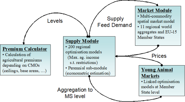
The CAPRI simulation tool is composed of a supply and market modules, interlinked with each other.
In the supply module, regional or farm type agricultural supply of crops and animal outputs is modelled by an aggregated profit function approach under a limited number of constraints: the land supply curve, policy restrictions such as sales quotas and set aside obligations and feeding restrictions based on requirement functions. The underlying methodology assumes a two stage decision process.
In the first stage, producers determine optimal variable input coefficients per hectare or head (nutrient needs for crops and animals, seed, plant protection, energy, pharmaceutical inputs, etc.) for given yields, which are determined exogenously by trend analysis (CAPRI reference scenario) and updated depending on price changes against the baseline. Nutrient requirements enter the supply models as constraints and all other variable inputs, together with their prices, define the accounting cost matrix.
In the second stage, the profit maximising mix of crop and animal activities is determined simultaneously with cost minimising feed and fertiliser in the supply models. Availability of grass and arable land and the presence of quotas impose a restriction on acreage or production possibilities. Moreover, crop production is influenced by set aside obligations and animal requirements (e.g. gross energy and crude protein) are covered by a cost minimised feeding combination. Fertiliser needs of crops have to be met by either organic nutrients found in manure (output from animals) or in purchased fertiliser (traded good).
A cost function covering the effect of all factors not explicitly handled by restrictions or the accounting costs –as additional binding resources or risk ensures calibration of activity levels and feeding habits in the base year and plausible reactions of the system. These cost function terms are estimated from ex post data or calibrated to exogenous elasticities.
Fodder (grass, straw, fodder maize, root crops, silage, milk from suckler cows or mother goat and sheep) is assumed to be non-tradable, and hence links animal processes to the crops and regional land availability. A detailed description can be found in Britz and Heckelei (1999). All other outputs and inputs can be sold and purchased at fixed prices. The use of a mathematical programming approach has the advantage to directly embed compensation payments, set-aside obligations, and sales quotas, as well as to capture important relations between agricultural production activities. Not at least, environmental indicators as NPK balances and output of gases linked to global warming are directly inputted in the system.
The market module breaks down the world into 40 country aggregates or trading partners, each one (and sometimes regional components within these) featuring systems of supply, human consumption, feed and processing functions. The parameters of these functions are derived from elasticities borrowed from other studies and modelling systems and calibrated to projected quantities and prices in the simulation year. Regularity is ensured through the choice of the functional form (a normalised quadratic function for feed, processing and supply and a generalised Leontief expenditure function for human consumption) and some further restrictions (homogeneity of degree zero in prices, symmetry and correct curvature). Accordingly, the demand system allows for the calculation of welfare changes for consumers, processing industry and public sector. Policy instruments in the market module include bilateral trade flows1). Tariff rate quotas (TRQs), intervention purchases and subsidised exports under the World Trade Organisation (WTO) commitment restrictions are explicitly modelled for the EU.
In the market module, special attention is given to the processing of dairy products. First, balancing equations for fat and protein ensure that these make use of the exact amount of fat and protein contained in the raw milk. The production of processed dairy products is based on a normalised quadratic function driven by the regional differences between the market price and the value of its fat and protein content. Then, for consistency, prices of raw milk are also derived from their fat and protein content valued with fat and protein prices.
The market module comprises of a bilateral world trade model based on the Armington assumption (Armington, 1969). According to Armington’s theory, the composition of demand from domestic sales and different import origins depends on price relationships according to bilateral trade flows. This allows the model to reflect trade preferences for certain regions (e.g. Parma or Manchego cheese) that cannot be observed in a net trade model.
The equilibrium in CAPRI is obtained by letting the supply and market modules iterate with each other. In the first iteration, the regional aggregate programming models (one for each NUTS 2 region or farm type) are solved with exogenous prices. Regional agricultural income is therefore maximised subject to several restrictions (land, fertiliser allocation, feed requirements, etc). After being solved, the regional results of these models (crop areas, herd sizes, input/output coefficients, etc.) are aggregated and enter a small, non-spatial multi-commodity module for young animal trade, as shown in Figure 12. In the second iteration, supply and feed demand functions of the market module are first calibrated to the results from the supply module on feed use and production obtained in the previous iteration. The market module is then solved at this stage (constrained equation system) and the resulting producer prices at Member State level transmitted to the supply models for the following iteration. At the same time, in between iterations, premiums for activities are adjusted if ceilings defined in the Common Market Organisations (CMOs) are overshot.
The implementation in CAPRI is based on a core module file gams/capmod.gms, which calls the different components of the system. The main input comes from the CAPRI database (COCO, CAPREG, GLOBAL), trends (CAPTRD) and baseline calibration parameters. The output of a scenario run is stored in a GDX file in folder output/results/capmod.
Module for agricultural supply at regional level
Basic interactions between activities in the supply model
There are two sources for interactions between activities in simulation experiments: the objective function and constraints. In the current version of CAPRI, the objective function does solve inter-activity terms for groups of arable crops, so that the major interplay is due to constraints. The interaction is best understood by looking at the first order conditions of a programming model including PMP terms:
\begin{equation} Rev_j = Cost_j+ac_j+\sum_k bc_{j,k}Levl_k+\sum_i^m\lambda_ia_{ij} \end{equation}
The left hand side (Rev) shows the marginal revenues, which are typically equal to the fixed prices times the fixed yields plus premiums. The right hand side shows the different elements of the marginal costs. Firstly, the variable or accounting costs (Cost) which are fix as they are based on the Leontief assumption. The term \( (ac_j+\sum_k bc_{j,k}Levl_k) \) shows the marginal non-linear costs, which are increasing with the activity levels. The cross effects are only introduced to let major arable crop groups interact, whereas for fruits & vegetables, permanent crops, grassland and the animal sectors, only diagonal terms are introduced. The methodology for the estimation of these terms is described in Jansson and Heckelei (2011).
The remaining term \( (\sum_i^m\lambda_ia_{ij}) \) captures the marginal costs linked to the use of exhausted resources and is equal to the sum of the shadow prices \lambda multiplied the per unit demand of resource i for activity j; the matrix A being again based on Leontief technology. The shadow values of binding resources hence are the drivers linking the activities.
The land balance plays a central role in the CAPRI supply model. The land shadow price appears as a cost in all crop activities including fodder producing ones, so that animals are indirectly affected as well. The second major link is the availability of not-marketable feeding stuff, and finally, less important, organic fertiliser.
The basic effects are best discussed with a simple example. Assume an increase of a per hectare premium for soft wheat, all other things unchanged.
- What will happen in the model? The increased premium will lead to an imbalance between marginal revenues (= yield times prices plus premium) and marginal costs (=accounting costs, ‘resource use cost’, non-linear costs). In order to close the gap, as marginal revenues are fixed, the area under soft wheat will be increased until marginal costs of producing soft wheat have increased to a point where they are again equal to marginal revenues. As the marginal costs linked to the non-linear cost function \( (ac_j+\sum_k bc_{j,k}Levl_k) \) are increasing in activity levels, increasing the area under soft wheat will hence reduce that gap. At the same time, as the land balance must be kept closed, other crop activities must be reduced. The non-linear cost function will for these crops now provoke a countervailing effect: reducing the activity levels of competing crops will lead to lower costs for these crops. With marginal revenues (Rev) and accounting costs (Cost) fixed, that will require the shadow price of the land balance to increase.
- What will be the impact on animal activities? Again, the shadow price of the land balance will be crucial. For activities producing non-marketable feed, marginal revenues are not defined as prices times yields, but as internal feed value times prices. The internal feed value is determined as the substitution value of non-marketable fodder against other feeding stuff, and depends on their nutrient content and further feed restrictions. Increasing the shadow price of land will hence either require decreasing other costs in producing fodder or increasing the internal marginal revenues. In other words, a high shadow price of land renders non-marketable fodder less competitive compared to other feeding stuff. As feed costs are – however very slightly – increasing in quantities fed per head, feed costs for animals will increase. But as there are several requirement constraints involved, some feeding stuff may increase and other decrease. Clearly, the higher the share of non-marketable fodder in the mix for a certain animal type, the higher the effect. As marginal feed costs will increase, and marginal revenues for the animal process are not changing, other marginal costs in animal production need to be reduced, and again the non-linear cost function will be the crucial part, as the marginal cost related to it will decrease if herd sizes drop.
To summarize the supply response, increasing premiums for a crop will hence increase the cropping share of that crop, reduce the share of other crops, increase the shadow price of land, lead to less fodder production, higher fodder costs and thus reduced herd size of animals.
- What will be the impacts covered by the market? The changes in hectares will lead to increased supply of the crop with the higher premium and less supply of all other crops at given prices, i.e. one upward and many downward shifts of the supply curves. Equally, supply curves for animal products will shift downwards. On the other hand, some feed demand curve will shift as well, some upward, other downward. These shifts will move the market module away from the former fixed points where market balances were closed. For the crop product with the increased premiums, increased supply plus some changes in feed will most probably lead to lower prices, whereas prices of other crops will most probably increase. That will require new adjustments during the next iteration where the supply models are solved, with to a certain extent countervailing effects.
Table 25: Overview on a regional aggregate programming model
| Crop Activities | Animal Activities | Feed Use | Net Trade | Constraints | |
| Objective function | + Premium – Acc.Costs – variable cost function terms | + Premium – Acc.Costs – variable cost function terms | - variable cost function terms for feeding | + Price | |
| Output | + | + | - | - | = 0 |
| Area | - | < = land supply | |||
| Set aside | +/- | = 0 | |||
| Quotas | - | - | < = Ref. Quantity | ||
| Fertilizer needs | - | + | + | = 0 | |
| Feed requirements | - | + | + | = 0 |
Detailed discussion of the equations in the supply model
The definition of the supply model can be found in ‘supply\supply_model.gms’
Feed block
The feed block ensures that the requirements of the animal processes in terms of feed energy and protein are met and links these to the markets and crop production decisions.
\begin{equation} \overline{AREQ}_{r,act,req} \overline{DAYS}_{r,act,req}= \sum_{feed} FEDNG_{r,act,feed} \overline{REQCNT}_{r,act,feed} \end{equation}
The left hand side captures the daily animal requirements (AREQ) for each region r, animal activity act and requirement AREQ multiplied with the days (DAYS) the animal is in the production process. Both are parameters fixed during the solution of the modelling system. The right hand side ensures that the requirement content of the actual feed mix represented by the feeding (FEDNG) of certain type of feed to the animals multiplied with the requirement content (REQCNT) in the regions covers these nutritional demands. Requirements and contents are specified in the feed calibration while production days are determined in the “COCO1” module. Total feed use (FEDUSE) in a region is defined as the feeding per head multiplied with the activity level (LEVL) for the animal activities:
\begin{equation} FEDUSE_{r,feed} = \sum_{aact} LEVL_{r,aact} FEDNG_{r,aact,feed} \end{equation}
Total feed use might be either produced regionally in the case of fodder assumed not tradable (grass, fodder root crops, silage maize, other fodder from arable land), or bought from the market at fixed prices.
Land balances and set-aside restrictions
The model distinguishes arable and grassland and comprises thus two land balances:
\begin{equation} \overline{LEVL}_{r,"arab"} \le \sum_{arab} LEVL_{r,arab} \end{equation}
\begin{equation} \overline{LEVL}_{r,"gras"} \le LEVL_{r,"grae"} + LEVL_{r,"grai"} \end{equation}
Both land balances might become slack if marginal returns to land drops to zero. For arable land, idling land not in set-aside (activity FALL) is a further explicit activity. For the grassland, the model distinguishes two types with different yields (GRAE: grassland extensive, GRAI: grassland intensive) so that idling grassland can be expressed of an average lower production intensity of grassland by changing the mix between the two intensities.
The model comprises a land use module with two major components:
- Imperfect substitution between arable and grass lands depending on returns to the two types of agricultural land uses.
- A land supply curve which determines the land available to agriculture as a function to the returns to land.
There are hence two further equations:
\begin{equation} \overline{LEVL}_{r,"uaar"} = \overline{LEVL}_{r,"arab"} +\overline{LEVL}_{r,"gras"} \end{equation}
And a further one which prevents numerical problems with the terms relating to land supply in the objective function
\begin{equation} \overline{LEVL}_{r,"uaar"} = 0.999 \overline{LEVL}_{r,"asym"} \end{equation}
Where “asym” is the land asymptote, i.e. the maximal amount of economically usable agricultural area in a region when the agricultural land rent goes towards infinity. For an application where the land market is used see Renwick et al. (2013).
Set aside policies have changed frequently during CAP reforms. The recent specification is covered in the context of the premium modelling in Section Premium module. The obligatory set-aside restriction introduced by the McSharry reform 1992 and valid until the implementation of the Luxembourg compromise of June 2003 has been explicitly modelled through this equation:
\begin{align} \begin{split} &LEVL_{r,"iset"} + LEVL_{r,"gset"} + LEVL_{r,"tset"} \\ &=\sum_{arab} LEVL_{r,arab}\left(1-NONS_{r,arab}\right ) \frac {1/100SETR_{r,arab}}{1- 1/100 SETR_{r,arab}} \end{split} \end{align}
LEVL_{r,“iset”}As seen from above, the model distinguishes between three types of obligatory set-aside: idling (ISET), for grass land use (GSET) and for forestation purposes (TSET). The share of so-called non-food production exempt from set-aside (NONS) for each activity and region is fixed and given.
The equation above is replaced for years where the Luxembourg compromise of June 2003 is implemented by a Member State, where the level of obligatory set-aside is fixed instead to the historical obligations.
For certain years of the McSharry reform, the total share of set-aside – be it obligatory or voluntary – on a list of certain crops was not allowed to exceed a certain ceiling. That restriction is captured by the following equation:
\begin{align} \begin{split} &LEVL_{r,"iset"} + LEVL_{r,"gset"} + LEVL_{r,"tset"}+ LEVL_{r,"vset"} \\ & \le \sum_{arab \wedge SETF_{r,arab}} LEVL_{r,arab}/\overline{MXSETA} \end{split} \end{align}
Fertilising block
As of CAPRI Stable Release 2.1, the fertilizer allocation was modified, and this section of the documentation updated. Notation has changed compared with previous versions of the model and documentation. Here, we represent the equations in more general mathematical notation, avoiding the long GAMS code names of the source code, in order to save space.
We distinguish the three macro-nutrients N, P and K. The supply and uptake of those nutrients are modelled in a uniform way, save for the fact that there is fixation and atmospheric deposition only of N.
Each crop has a requirement per hectare, calculated based on the yield. Yields are exogenous from the vantage point of the producer, but there are alternative technologies available for each cropping activity, and a separable, i.e. handled outside of the optimization model, relation between prices and optimal yields.
From the basic nutrient requirement we first deduct the rate of biological fixation (only for nitrogen and selected crops). The remainder is inflated by a (calibrated) factor and additive term of over-fertilization, and then scaled with a soil-specific factor (only for nitrogen), to arrive at the total amount of nutrients that need to be supplied to the crop. This is the left hand side of Equation 96 
Nutrient supply, shown on the right handside, comes from mineral fertilizer, manure, crop residues and atmospheric deposition. Mineral fertilizer may have ammonia losses during application. For manure, there are both losses and inefficiencies. When manure is applied to crops, there is an efficiency factor applied to the nutrient content (denoted by ϕ_(r,“excr”, n) ), corresponding to the Fertilizer Value (FV) of manure relative to mineral fertilizer. The efficiency factor is a key parameter of interest in simulations carried out in some studies. Crop residues can be re-distributed among crop groups for annual arable crops but not for grassland and permanent crops, where it stays with the crop that produced it. For crop residues there is both a loss rate and a fertilizer value.
\begin{align}
\begin{split}
&\sum_{i \in I \, j,k} \left[ levl_{rik} \left ( ret_{rni} (1-biofix_{rni}) \lambda_{rnik}^{prop} + \lambda_{rni}^{const} \right ) soil_{rn} \, yf_{rnik} \right ] \\
& = fmine_{rni}(1-loss_{rn}) +fexcr_{rni} \phi_{r,excr,n} +(1-isPerm_j)fcres_{rni}(1-loss_{rn})\phi_{r,cres,n}\\
& + isPerm_j \sum_{ i \in I \, j,k} levl_{rik}res_{rni}(techf_{rink}+1)(1-loss_{rn})\phi_r,cres,n \\
& \forall r,n,j
\end{split}
\end{align} 
Indices:
\(r\) = region
\(i\) = crop
\(j\) = crop group
\(k\) = technological crop option (high/low yield)
\(n\) = nutrient (N/P/K)
\(isPerm_j\) = indicates that crop group \(j\) contains permanent crops
Endogenous choice variables:
\(levl_{rik}\) = Area (ha) of each crop \(i\) and technology \(k\) in region \(r\).
\(fmine_{rnj}\) = Application of mineral fertilizer \(n\) to crop group \(j\) in region \(r\).
\(fexcr_{rnj}\) = Application of manure \(n\) to crop group \(j\) in region \(r\).
\(fcrex_{rnj}\) = Allocation of crop residue \(n\) to crop group \(j\) in region \(r\).
Parameters:
\(ret_{rni}\) = Retention (uptake) of nutrients by the crop
\(res_{rni}\) = Crop residues output
\(biofix_{rni}\) = Biological fixation, share (only for N and selected crops)
\(λ_{rnik}^{prop} \) = Over-fertilization factor, calibrated
\(λ_{rni}^{const} \) = Over-fertilization term, calibrated
\(soil_{rn}\) = Soil factor
\(yf_{rnik}\) = Yield factor for technologies
\(loss_{rn}\) = Loss rate
\(ϕ_{r",excr" ,n}\) = Nutrient availability ratio for manure
\(ϕ_{r,"cres" ,n}\) = Nutrient availability ratio for crop residues
The reader may have noted that there is no loss rate for manure in the Equation 96 
The model contains three types of manure: N-manure, P-manure and K-manure. From an agricultural point of view this may seem odd. It might be more intuitive to think of one type of manure per animal category. The motivation is to keep the system simple and flexible. With the present representation, where each animal category supplies N, P, and K-manure, the number of manure classes can be limited and yet the unique mix of nutrients from each animal category can be defined.
The supply of each manure type is collected in a “pool” for each regional farm model, i.e. for each NUTS2 region. Regions within a member state may trade manure, subject to a cost. The supply in the pool plus the traded quantities has to be distributed to the crops in the region, i.e. there is an equality-restriction in place. This is handled in the equations “FertDistExcr_” and “ManureNPK_”. Note that fertilizer flows are measured in tons, for the sake of scaling, whereas other total quantities in CAPRI are measured in 1000 tons. Hence the factors 1000 and 0.001.
\begin{equation} \sum_j fexcr_{rnj}= 1000 v\_ManureNPK_{rn} \end{equation}
\begin{equation} v\_ManureNPK_{rn} + \sum_s T_{rs}nutshr_{rn} = 0.001 \sum_{i\in Anim_j,k} levl_{rik}o_{rnik}(1-loss_{rin}) \quad \forall r, n \end{equation}
where
\(o_{rnik}\) is the output of manure nutrient \(n\) from animal type \(i\) using technology \(k\) in region \(r\),
\(nutshr_{rn}\) is the average content of each nutrient in the regional manure pool,
\(T_{rs}\) is the quantity of manure traded from \(r\) to \(s\),
\(isAnim_{i}\) indicates that activity \(i\) is an animal production activity
Equation “FertDistMine_” allocates total mineral fertilizer sales to the crops / group of crops.
\begin{equation} \sum_j fmine_{rnj} = -netPutQuant_{rn} \end{equation}
Finally, crop residues and atmospheric definition are distributed in equation “FertDistCres_”.
\begin{equation} \sum_j fcers_{rnj} = \sum_{i \notin isPerm_j,k} levl_{rik}res_{rni}(techf_{rink}+1) \end{equation}
One flow from a source s={“mine” ,“cres” ,“excr” } to a sink j={“crop groups”} can in general be anything from zero and upwards. The nutrient balance equations above do not uniquely determine each flow of nutrients from sources to sinks, but it is indeed possible that in one simulation, say, a particular crop group gets much crop residues and little manure, whereas the opposite holds in the next simulation. The total balances will hold equally well in either situation, and the profits will not be affected since the same total amount of mineral fertilizer is purchased, but we do have a stability problem for the model. Furthermore, the different nutrient flows may influence the greenhouse gas emission coefficients of crops (if e.g. the emissions of enteric fermentation follows the manure to the crops). The problem is under-determined, or ill-posed.
To resolve the ill-posedness of the fertilizer distribution, we propose a probabilistic approach. This means that we do not introduce any additional economic model for the allocation that somehow makes increasing fertilizer flows more expensive. Instead, we assume that whatever the reasons the farmers have for choosing a particular distribution, those reasons are similar in two simulations, and therefore the fertilizer flows are also similar. Thus, a larger deviation from some reference flows is deemed improbable, albeit not costlier than the situation with the reference flows.
To develop this probabilistic model, we assume that the decisions of the farmer are separable and taken in two steps: first, the farmer decides about the cropping plan and just ensures that the total amount of fertilizer available is sufficient. This is called the outer model. Then, a statistical model is solved that finds the most probable fertilizer flows out of the continuum of possible ones. This is called the inner model. The structure with outer and inner models makes the problem a bi-level programming one.
To implement the bi-level programming problem in a way that does not change the present structure of the model (with just one optimization solve of the representative farm model) we implement the inner model by its optimality conditions. By carefully choosing the proper probability density functions we ensure that no complementary slackness conditions are needed, so that the inner model is simple to solve. For this the gamma density function is very suitable, as it has a support from zero to infinity, with a probability that goes towards zero as the random variable goes to zero.
The parameters of the gamma function are determined in the calibration step, described further below, and then kept constant in simulation. The gamma density function for some random variable x has the form
\begin{equation} p(x|\alpha,\beta) = \frac {\beta^{\alpha}}{\Gamma(\alpha)}x^{\alpha-1}e^{-\beta x} \end{equation}
where Γ(α) is the gamma function, and α and β are parameters that determine the shape of the density function. The gamma density is nonlinear, and the joint density, being the product of the densities of all nutrient flows, is even more so. In order to reduce nonlinearity we note that are interested in finding the highest posterior density, i.e. maximizing a joint density function, and since the maximum is invariant to monotonous positive transformations we compute the logarithm of the joint density, which will be the sum of terms like the following (the constant term has been omitted since it also does not influence the optimal solution for x):
\begin{equation} log \, p(x|\alpha,\beta) \propto (\alpha-1)log \, x-\beta x \end{equation}
Maximization of the logged density under the constraints that the nutrient balance restrictions of the supply modes have to be met gives a set of equations that define explicit and unique fertilizer flows, where v are the Lagrange multipliers of the source-pool restrictions and u the Lagrange multipliers of the nutrient balance equation.
\begin{equation} \text{FOC w.r.t. manure use:} \\ \frac {\alpha_{r,excr,nj}-1}{fexcr_{rnj}} - \beta_{r,excr,nj} - v_{r,excr,n}+\phi_{r,excr,n}u_{rnj} = 0 \end{equation}
\begin{equation} \text{FOC w.r.t. crop residues use:} \\ \frac {\alpha_{r,cres,nj}-1}{fcres_{rnj}} - \beta_{r,cres,nj} - v_{r,cres,n}+(1-loss_{rn}\phi_{r,excr,n}u_{rnj} = 0 \forall j\notin isPerm_j \end{equation}
\begin{equation} \text{FOC w.r.t. mineral feritilzer use:} \\ \frac {\alpha_{r,mine,nj}-1}{fmine_{rnj}} - \beta_{r,mine,nj} - v_{r,mine,n}+(1-loss_{rn}u_{rnj} = 0 \end{equation}
The system of FOC contains expressions of the type \(1/fmine\) which is likely to impair performance as the second derivatives are not constant (CONOPT computes second derivatives). Therefore, the first term in each FOC was turned into a new variable \(z\) defined as \( z_{r,"excr" ,nj}fexcr_{r,"excr" ,nj}=\alpha_{r,"excr" ,nj}-1\), and similar for each source, which is a quadratic expression.
Balancing equations for outputs
Outputs produced must be sold – if they are tradable across regions – or used internally, as in the case of young animals or feed.
\begin{equation} \sum_{act}Levl_{r,act}OUTP_{r,act,o}=NETTRD_r^{o\notin fodder}+YANUSE_r^{o\notin oyani} +FEDUSE_r^{o\in fodder} \end{equation}
In the case of quotas (milk, for sugar beet) the sales to the market may be bounded (noting that NETTRD = v_netPutQuant in the code):
As described in the data base chapter, the concept of the EAA requires a distinction between young animals as inputs and outputs, where only the net trade is valued in the EAA on the output side. Consequently, the remonte expressed as demand for young animals on the input side must be mapped into equivalent ‘net import’ of young animals on the output side:
\begin{equation} \sum_{aact}Levl_{r,aact}I_{r,aact,yani}=YANUSE_r^{oyani \leftrightarrow iyani} \end{equation}
In combination with the standard balancing equation shown above, the NETTRD variable for young animals on the output side becomes negative if the YANUSE variable for a certain type of young animals exceeds the production inside the region.
The objective function
The objective function is split up into the linear part, the one related to the quadratic cost function for activities, and the quadratic cost function related to the feed mix costs:
\begin{equation} OBJE=\sum_r LINEAR_r+QUADRA_r+QUADRF_r \end{equation}
The linear part comprises the revenues from sales and the costs of purchases, minus the costs of allocated inputs not explicitly covered by constraints (i.e. all inputs with the exemptions of fertilisers, feed and young animals) plus premiums:
\begin{equation} LINEAR_r= \sum_{io} NETTRD_{r,io} \overline{ PRICE}_{io}+ \sum_act LEVL_{r,act}\left (\overline{PRME}_{r,act}-\overline{COST}_{r,act}\right) \end{equation}
The quadratic cost function relating to feed is defined as follows:
\begin{equation} QUDRAF_r = \sum_{aact,feed} \left[ \begin {matrix} LEVL_{r,aact}FEDNG_{r,aact,feed} \\ (a_{r,aact,feed}+ 1/2b_{r,aact,feed}FEDNG_{r,aact,feed}) \end{matrix} \right] \end{equation}
The marginal feed costs per animal increase hence linearly with an increase in the feed input coefficients per animal. It should be emphasised that this is the main mechanism that “stabilises” the feed allocation by animals. The two balances on feed energy and protein alone would otherwise leave the feed allocation indeterminate and give a rather “jumpy” simulation behaviour.
There is another more complex PMP term (equation quadra_ in supply_model.gms, not reproduced in this section) quadratic in activity levels and differentiated by the two technologies that “stabilises” the composition of activites according to previous econometric estimates or default assumptions.
A final term relates to the entitlements introduced with the 2003 Mid Term reviews. If those entitlements are overshot, a penalty term equal to the premium paid under the respective scheme (regional, historical etc.) is subtracted to the objective. Accordingly, the marginal premium for an additional ha above the entitlement ceiling is zero.
Sugar beet (M. Adenäuer, P. Witzke)
The Common Market Organisation (CMO) for sugar regulates European sugar beet supply with a system of production quotas, even after the significant reforms of 2006, up to year 2017 when the quota system expired. Before that reform, two different quotas had been established subject to different price guarantee (A and B quotas, qA and qB). Beet prices were depending on intervention prices and levies to finance the subsidised export of a part of the quota production to third countries. Sugar beets produced beyond those quotas (so called C beets) were sold as sugar on the world market at prevailing prices, i.e. formally without subsidies. However, a WTO panel initiated by Australia and Brazil concluded that the former sugar CMO involved a cross-subsidisation of C-sugar from quota sugar such that all exports of C sugar was also counted in terms of the EU’s limits on subsidised exports. As a consequence, this outlet for EU surplus production was closed. The reformed CMO therefore does not allow any exports beyond the Uruguay round limits. Instead, processing of beets to ethanol emerged as a new outlet that economically plays a similar role as former C beet production: It offers an outlet for high production quantities that exceed the quota limits of farmers, but at a reduced price. Basically, farmers face a kinked beet demand curve that potentially involved three price levels:
- A-beets receiving the highest price derived from high sugar prices (and before the 2006 reform less a small levy amount)
- B-beets receiving a lower price as the applicable levies were higher before the reform. However, the 2006 reform eliminated the distinction of A and B quotas. Furthermore, the sugar industry applied a pooling price system in many MS that also eliminated the distinction between A and B beets.
- C-beets receiving the lowest price, formerly derived from world market sugar prices, now derived from ethanol prices.
The high price sector covers for farmers at least the farm level quota endowment. However, the sugar industry may grant high prices also for a limited, “desirable” over-quota production, for example to avoid bottlenecks in sugar or ethanol production. This has been the case in some EU countries before the reform (so-called “C1 beets”) and it is also current practice (see, for example http://www.liz-online.de).
Considering a kinked demand curve and in addition yield uncertainty renders the standard profit maximisation hypothesis inappropriate for the sugar sector (at least). The CAPRI system therefore applies an expected profit maximisation framework that takes care for yield uncertainty (see Adenäuer 2005). The idea behind this is that observed C sugar productions in the past are unlikely to be an outcome of competitiveness at C beet prices rather than being the result of farmers’ aspirations to fulfil their quota rights even in case of a bad harvest. This approach essentially assumes that the “behavioural quotas” of farmers may exceed the “legal quotas” (derived from the sugar CMO) by some percentage. This percentage reflects in part the pricing behaviour of the regional sugar industry, but it may also depend on farmers expectations on the consequences of an incomplete quota fill. These aspects may be captured with the following specification of expected sugar beet revenues that substitute for the expression \(NETTRD_{r,io} \; PRICE_{io} \) (if \(io=SUGB\)) in equation below:
\begin{align} \begin{split} SegbREV_r & = p^A NETTRD_{r,SUGB} \\ & - \left( p^A-p^B\right) \left [ \begin{matrix} (1-CDFSugb(q^A))(NETTRD_{r,SUGB}-q^A) \\ + (\sigma^S)^2 PDFSugb(q^A) \end{matrix} \right] \\ & -\left(p^B-p^C\right) \left [ \begin{matrix} (1-CDFSugb(q^A+B))(NETTRD_{r,SUGB}-q^A+B) \\ + (\sigma^S)^2 PDFSugb(q^A+B) \end{matrix} \right] \end{split} \end{align}
Where \(PDFSugb_r\) and \(CDFSugb_r\) are the probability res. cumulated density functions of the NETTRD variable with the standard deviation \(\sigma^S\). \(\sigma^S\) is defined as \(NETTRD_{r,SUGB} * VCOF_r\), where the latter is the regional coefficient of yield variation estimated from FADN. \({p^ABC}\) are the prices for the three different types of sugar beet which are exogenous and linked to the EU and world market prices for sugar. The quotas \(q^A\) and \(q^{A+B}\) used in Equation 111 
\begin{align} \begin{split} p^A &= legalqout^A \cdot scalefac \\ & = legalqout^A \cdot \left(\frac{NETTRD_{SUGB}^{cal}}{legalqout^A} \right )^{0.8} \end{split} \end{align}
The scaling factor to map from the legal quota legalquotA (as the B quota has been eliminated in the sugar reform, it holds that \(q^A = q^{A+B}) \)to the behavioural quota qA depends on the projected sugar beet sales quantity in the calibration point \(NETTRD_{SUGB}^{cal} : For a country with a high over quota production (say 40%) we would obtain a scaling factor of 1.31, such that this producer will behave like a moderate C-sugar producer: responsive to both the C-beet prices as well as to the quota beet price (and the legal quotas). Without this scaling factor, producers with significant over quota p roduction, like France and Germany, would not show any sizeable response to a 10% cut of either the legal quotas or the quota price (at empirically observed coefficients of variation). As it is likely that the profitability of ethanol beets benefit from cross-subsidisation from the quota beets such a zero responsiveness was considered implausible. ===Update note=== A number of recent developments are not covered in the previous exposition of supply model equations -A series of projects have added a distinction of rainfed and irrigated varieties of most crop activities which is the core of the so-called “CAPRI-water” version of the system((A more complete presentation is given in [[https://ec.europa.eu/jrc/en/publication/eur-scientific-and-technical-research-reports/extension-capri-model-irrigation-sub-module]].)). -Several projects have added endogenous GHG mitigation options((These are most completely included in the “trunk” version of the CAPRI system. For details, see, for example, [[http://publications.jrc.ec.europa.eu/repository/bitstream/JRC101396/jrc101396_ecampa2_final_report.pdf]].)) -Several new equations serve to explicitly represent environmental constraints deriving from the Nitrates Directive and the NEC directive((These are most completely included in the “trunk” version of the CAPRI system but developments are still ongoing.)). -A complete area balance monitoring the land use changes according to the six UNFCCC land use types (cropland, grassland, forest land, wetland, settlements, residual land) has been introduced for carbon accounting ====Calibration of the regional programming models==== Since the very first CAPRI version, ideas based on Positive Mathematical Programming were used to achieve perfect calibration to observed behaviour – namely regional statistics on cropping pattern, herds and yield – and data base results as the input or feed distribution. The basic idea is to interpret the ‘observed’ situation as a profit maximising choice of the agent, assuming that all constraints and coefficients are correctly specified with the exemption of costs or revenues not included in the model. Any difference between the marginal revenues and the marginal costs found at the base year situation is then mapped into a non-linear cost function, so that marginal revenues and costs are equal for all activities. In order to find the difference between marginal costs and revenues in the model without the non-linear cost function, calibration bounds around the choice variables are introduced. The reader is now reminded that marginal costs in a programming model without non-linear terms comprise the accounting cost found in the objective and opportunity costs linked to binding resources. The opportunity costs in turn are a function of the accounting costs found in the objective. It is therefore not astonishing that a model where marginal revenues are not equal to marginal revenues at observed activity levels will most probably not produce reliable estimates of opportunity costs. The CAPRI team responded to that problem by defining exogenously the opportunity costs of two major restrictions: for the land balance and for milk quotas. The remaining shadow prices mostly relate to the feed block, and are less critical as they have a clear connection to prices of marketable feed as cereals which are not subject to the problems discussed above. ====Estimating the supply response of the regional programming models==== The development, test and validation of econometric approaches to estimate supply responses at the regional level in the context of regional programming models form an important task for the CAPRI team. Up to now, there is still no fully satisfactory solution of the problem, but some of the approaches are discussed in here. The two possible competitors are standard duality based approaches with a following calibration step or estimates based directly on the Kuhn-Tucker conditions of the programming models. Both may or may not require a priori information to overcome missing degrees of freedom or reduce second or higher moments of estimated parameters. The duality based system estimation approach has the advantage to be well established. Less data is required for the estimation, typically prices and premiums and production quantities. That may be seen as advantage to reduce the amount of more or less constructed information entering the estimation, as input coefficients. However, the calibration process is cumbersome, and the resulting elasticities in simulation experiments will differ from the results of the econometric analysis. The second approach – estimating parameters using the Kuhn-Tucker-conditions of the model – leads clearly to consistency between the estimation and simulation framework. However, for a model with as many choice variables as CAPRI that straightforward approach may require modifications as well, e.g. by defining the opportunity costs from the feed requirements exogenously. The dissertation work of Torbjoern Jansson (Jansson 2007) focussed on estimating the CAPRI supply side parameters. The results have been incorporated in the current version. The milk study (2007/08) contributed additional empirical evidence on marginal costs related to milk production (Kempen et al. 2011) ====Price depending crop yields and input coefficients ==== Let Y denote yields and j production activities. Yield react via iso-elastic functions to changes in output prices \begin{equation} log(Y_j)=\alpha_j+\epsilon_j \, log(p_o) \end{equation}
The current implementation features yield elasticities for cereals chosen as 0.3, and for oilseeds and potatoes chosen as 0.2. These estimates might be somewhat conservative when compared e.g. with Keeney and Hertel (2008). However, in CAPRI they relate to small scale regional units and single crops, and to European conditions which might be characterized by a combination of higher incentive for extensive management practises and dominance of rainfed agriculture where water might be a yield limiting factor.
Currently, the code is set up as to only capture the effect of output prices. However, in order to spare calculation of the constant terms α, the actual code implemented in ‘endog_yields.gms’ change the yields iteratively in between iterations t, using relative changes:
\begin{equation} Y_{j,t}=Y_{j,t-1}^{[\epsilon_jlog \frac{p_o,t-1}{p_t}]} \end{equation}
Premium module
Overview
For the European Union, the CAPRI programming models cover in rich detail the different coupled and de-coupled subsidies of the so-called first Pillar 1 of the CAP, as well as major ones from Pillar 2 (i.e., Less Favoured Area support, agri-environmental measures, Natura 2000 support). The interaction between premium entitlements and eligible hectares for the Single Farm Payment (SFP) of the CAP is explicitly considered, as are the different national SFP implementations, possibly remaining coupled payments (previously under article 68 of Council Regulation (EC) No. 73/2009, from 2014 as “Voluntary Coupled Support”).
Decoupled payments – as with other premium schemes of the CAP from the present and past – are simulated in CAPRI relatively closely to their definition in existing legislation. The rather high dis-aggregation of the model template regarding production activities and the resolution by farm types inside of NUTS 2 regions clearly eases that task. Currently, 260 different voluntary coupled support schemes are implemented, in addition to decoupled income support (Basic Payment Scheme, BPS).
The payments – both in reality and in the model – tend to be defined in a cumulative manner. In 1992, the direct payments were introduced based on the previous price support levels multiplied by regional historic reference yields. The payments therefore became regionally differentiated. In the subsequent decoupling under Agenda 2000 and the following reforms, the single farm payments were defined based on the payments that each farm had previously received. The payments got very different expressed per hectare for farms in high yield regions versus low yield regions and for farms that had held animal payments versus arable farms. Then, the 2013 reforms introduced convergence of payment rates, both across farms (internal convergence) and between member states (external convergence). CAPRI reflects these incremental reforms, so that the payment rates in the most recent reform are based on coupled payments from MacSharry times.
Given that each reform has added complexity to the previous system, so too has the premium module of CAPRI grown to maintain the capacity to model previous reforms while allowing novel features such as greening to be introduced. Nevertheless, two generic features can be distinguished, that form the basis for many payments: the basic concept of a premium payment, and the idea of payment entitlements. Those are treated in separate sections here. Then, we proceed to describe the incremental reforms of the first pillar of the CAP, starting with the most recent, and the implementation of selected second pillar payments. Finally, we discuss certain elements relating to the reporting of premium payments, most notably the financing over different budgets.
Basic concept
In the CAPRI supply module, premiums are always paid per activity level (per hectare or per animal) basis. They can be differentiated by the low and high yield variant of each crop activity. The premiums are calculated in the premium module from different premium schemes.
A premium scheme (such as DPGRCU for the Grandes Cultures premiums after the Fischler reform) is a logical entity which encompasses:
- A specific application type (defining the basis for the payment amount)
- a region or regional aggregate to which it is applied,
- Possible ceilings in entitlements (CEILLEV) and in value (CEILVAL)
- Payment rates for possibly several lists of activities (such as PGGRCU for all types of Grandes Cultures or PGPROT for protein crops).
- Optionally an indication of the marginal payment when a ceiling is reached
- Optionally a modifier for different amounts per technology
The schemes provide many-to-many mappings between policy instruments and agricultural activities: each scheme can apply to many different activities – with possibly differentiated rates – and each activity can draw support from different schemes.
The application type defines how the nominal amount (called PRMR) is applied. Currently, the following application types are supported:
- perLevl = per ha or head
- perSlgtHd = per slaughtered head
- perYield = per unit of main output
- perHistY = per historic yield
- perLiveStockUnit = per livestock unit
- noDirPay = Norwegian direct payment
- noPriceSup = Norwegian price support
The application type points to a factor by which the nominal amount PRMR (for PRemiuM in Regulation) is converted to a declared value per hectare or head (PRMD). For perLevl, the factor is unity (it is already per hectare), but for instance for perYield, the amount is interpreted as a payment per unit of main output. That is used for the Nordic Aid Scheme for dairy cows in the northmost parts of Europe and for coupled payments in Norway.
Each payment is defined for one or seveal groups of activities, functioning as lists of eligible activities. Additionally, the payment can be applied in different rates to the high and low yield variant, to model e.g. an extensification premium.
Each premium scheme also has up to two ceiling values:
- ceilLev = Ceiling on LEVL, i.e. the number of hectares or heads
- ceilVal = Ceiling on the total budget (envelope) spent on the scheme
In the basic setting, the ceilings work as the old Grandes Cultures payment: if the total quantity (hectares or amount) exceeds the ceiling, then the payment to each farmer is reduced so that the ceilings are respected. This means that the marginal payment is somewhat reduced but does not become zero. For some other schemes, such as the Basic Payment Scheme of the CAP 2014-2020, there is a hard limit on the number of payment entitlements, so that the marginal payment becomes zero if the ceiling is overshot. That behaviour can be triggered by including the payment scheme set element in a special set PSDPAY_cutEndog, as in the following example from “pol_input\mtr_until2013.gms”.
PSDPAY_cutEndog(“DPSAPS”) = YES;
PSDPAY_cutEndog(“DPREG”) = YES;
PSDPAY_cutEndog(“DPFRMS”) = YES;
PSDPAY_cutEndog(“DPFRMF”) = YES;
PSDPAY_cutEndog(“DPGREEN”) = YES;
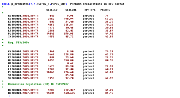
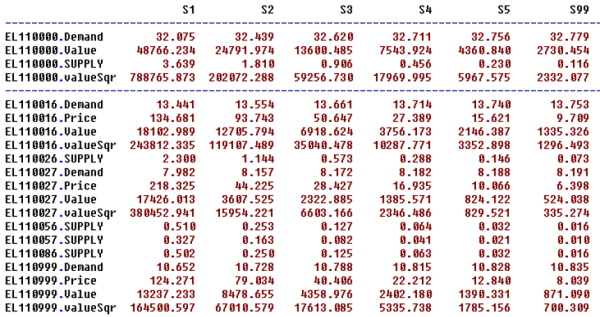
The following figure shows the technical implementation at an example:
Figure 14: Example of technical implementation of a premium scheme
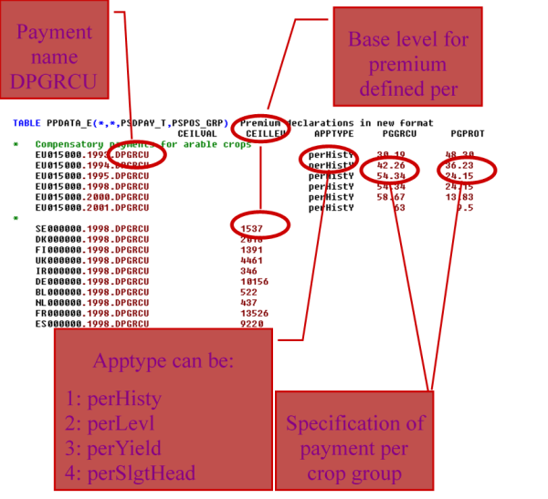
Source: CAPRI Modelling System. Note: The parameter PPDATA_E is now called p_premDataE.
The sets of payments, exemplified by DPGRCU in the figure, and the activity groups, exemplified by PGGRCU and PGPROT are defined in the file policy\policy_sets.gms. Since this is a “static” GAMS file used in any simulation, it contains the gross list of all policies that currently can be simulated, including legacy ones. In order to work efficiently with the acronyms which define the application types, these are converted to numerical attributes as shown below (‘policy\policy.gms’):
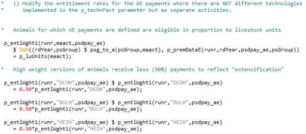
CAPRI also provides the possibility to incentivise extensification or intensification via the payments. Most production activities come in technological variants, by default one higher yielding and one lower yielding one, and those variants can be eligible to different rates of premium payments. This is used for instance in the implementation of agri-environmental schemes in the file policy\rd_logic.gms as shown in the figure below. The parameter p_technFact is the standard coefficient that modifies the technology of the production activities in CAPRI. In the figure below, the two statements change the rate of premium payments for the set of currently active regions (rs), for all model activities (MPACT), for all agri-environmental schemes (psdpay_ae) with different rates for technology T1 (high yield) and T2 (low yield) in the case where T2 exists. +0.5 for T2 means that the premium payment in the model becomes the nominal rate times (1 + 0.5), i.e. 50% higher, whereas the -0.5 for T1 means that the premium payment in the model becomes the nominal rate times (1 – 0.5), i.e. 50% lower. This approximates the stylized fact that agri-environmental schemes, which in reality consist of a wide range of measures, in general favour extensive technologies (see section on Pillar II payments below).
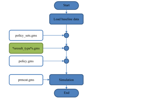
The general flow of logic inside of CAPRI (inside the model file capmod.gms) as regards premiums is shown in the following figure. The process starts by loading baseline data, including calibrated behavioural parameters. That data set represents an equilibrium situation for the policy (premiums) that were used in the baseline generation process.
After loading data, the file with declarations of all available premium schemes et cetera (policy_sets.gms) is loaded. The particular policy to use in the present simulation is contained in the policy file with the name defined by the placeholder (environment/macro variable) %result_type%. This string will also be part of the file name used for the simulation results.
The premiums defined in the policy file is processed by the file policy.gms. That processing implies a translation of the regulation-like definitions used in the policy file to parameters useful for CAPRI.
Within the simulation algorithm itself, a special file called prmcut.gms is called repeatedly, with the purpose to cut effective premium rates paid in case any ceiling is overshot, so that budgets are respected.
Figure 15: General flow of logic of CAPRI model as regards premiums
Generally, all attributes for a premium scheme are mapped down in space, e.g. from EU27 to EU 27 member states, from countries to NUTS1 regions inside the country, from there to the NUTS2 regions inside the NUTS1, and from NUTS2 regions to the farm types in a NUTS2 region (see ‘policy\policy.gms’), e.g.
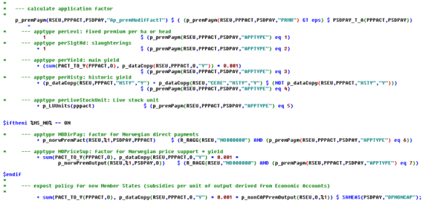
In order to map the premium rate as defined in a legal text into one paid out on a per-activity basis, the relevant activity based attribute matching the application type is set to a premium modification factor (“Ap_premModfFactT”) as shown below:
The actually declared premium per activity unit (ha, [1000] [slaughtered] heads) is then the multiplication of the premium rate and that modification factor. For crops, the unit of the resulting entries are current € per ha, for animal, it depends on the exact definition of the activity level (per [1000] [slaughtered] heads).
These declared rates can hence be aggregated to higher regional units using the activity levels as weights, e.g. from farm types to NUTS2:
Before the supply module is started between iterations, the current activity levels and premiums paid out are summed up for each scheme and regional level where ceilings in levels or value are defined. If one of the aggregated sums exceeds the ceilings, all premium rates for the scheme are cut proportionally to fit under the tighter of the two envelops:
From the declared rates and these cut factors, the actually paid premiums are defined:
The indivudal premiums from each premium scheme are then added up to arrive at one average rate for each activity which enters the objective function of the supply model, the data base and post-model reporting:
An example of a payment with a ceiling
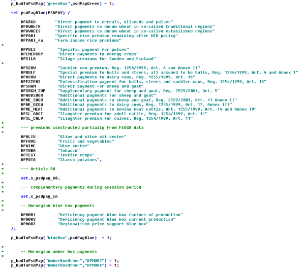
We explain the different elements and steps in the following based on an example of the slaughter premium for adult cattle of 80 EURO per slaughtered head in Latvia, defined in 2004. The following screen shot comes from the policy file gams\pol_input\mtr_until2013.gms, with some lines hidden.
- The application type defines the criterion upon which the payment depends, in the case of the slaughter premium it is defined per slaughtered head.
- The regulation premium rate (PRMR) is the default (maximum, uncut) amount of the premium according to regulatory texts, for all activities coverd by the premium group (here PGMEAT) and regions for which the premium is defined. In the example, this means that it is 80 EURO for the group of activities PGMEAT, which is dairy cows, suckler cows, male adult cattle and fattened heifers, in Latvia (LV000000). This is defined in a hierarchical way: if it is set to 80 EURO for the EU and not set at all at lower regional level, the 80 EURO are mapped down to all sub regions by the program. The program also lets you define groups of activities that are linked to the premium. In this case a group PGMEAT has been defined which contains the relevant animals (set s_PSGRP(*) in the file ‘policy_sets.gms’).
- The declared amount in the activity definition of CAPRI (per ha, per head, per 1000 heads) way that the amount PRMR should be applied or declared in CAPRI is called declared premium (PRMD) and applies per head or hectare. In our example, the regulation says that 80 EURO should be paid when the animal is slaughtered. That means that in order to get the amount per living animal and year, the 80 EUROs have to be multiplied by the frequency with which the animal is slaughtered. For male beef cattle it is 1/year whereas it for dairy cows is something like 1/5 years. These numbers come from the CAPRI database.
- Regional ceiling, expressed in maximum number of premiums paid and/or total payment in EURO. In the example with the slaughter premiums, this is used to set a national ceiling limiting the total amount spent on slaughter premiums to 9.946 million euro. There can be additional ceilings at other regional levels, and the most strongly binding is always the one that limits payments.
Those four pieces of information are generally easily accessible without further processing from the regulatory texts. Starting with PRMR and APPTYPE (information pieces 1 and 2 above), it is possible to calculate (3), PRMD, the amount of premium per head or hectare that would be paid if there were no (active) ceiling. These preparatory calculations, e.g. the hierarchical break down from higher to lower regional level and from activity groups to individual activities, as well as the calculations of PRMD from PRMR (using APPTYPE) is carried out in a file called ‘policy\policy.gms’ as shown above.
For most premiums in CAP there are ceilings, which if they are binding decrease the average amount of premiums actually paid (effective premium, PRME) per head or hectare. As discussed, due to the different kind of ceilings, the reduction of premiums and the treatment of PRME can only be done endogenously during the simulations depending on the simuled production patterns.
How is this problem solved in CAPRI? The effective premium (PRME) is exogenous during the optimisation of the supply model2), but adjusted iteratively between the main model iterations. So, for most premium schemes, the premium level is constant in the objective function and hence the model does not realise that the marginal premium payment is zero as soon as the ceiling is reached. Technically, the iterative adjustment of the effective premiums PRME is handled in a file called ‘policy\premcut.gms’ for “premium cut”. That reasoning is correct as long as the ceiling is not farm specific.
In each iteration, once all regional model are solved, the program adds up total number of premium units (hectares or heads for which it is paid) that belong to each ceiling. In most cases this simply means summing up number of animals or hectares of the activities for which each premium applies. This is also multiplied with the declared amount PRMD to get the total payment which would be paid if it would not be cut. For each premium this is compared to the ceilings defined (total level with the level ceiling and total amount with the value ceiling) and a “cut factor” is calculated, which defines how much the premium has to be reduced in order to fit under all ceilings. Then PRMD is multiplied by this factor to get the effective premium (PRME) for the next iteration.
Pillar I
The MTR-reform and the health check
On 26 June 2003, EU farm ministers adopted a further fundamental reform of the Common Agricultural Policy (CAP). The central element of the 2003 CAP reform was the introduction of the so-called single payment scheme (SPS). The SPS is based on payments entitlements linked to eligible land, but decoupled from production. However, to avoid abandonment of production, Member States could still choose to maintain a limited link between subsidy and production under well defined conditions and within clear limits. Moreover, these new “single farm payments” would be linked to environmental, food safety and animal welfare standards and obligations.
Key elements of the 2003 CAP reform were:
- A single farm payment for EU farmers, independent from production; limited coupled elements may be maintained to avoid abandonment of production;
- land receiving payments should be kept in good agricultural and environmental condition (G.A.E.C). “Good agricultural condition is generally interpreted to mean that the land will not be abandoned and environmental problems such as erosion will be avoided” this requirement could be interpreted as re-establishing the link between the payment and the factors of production employed (land management practices) and ultimately current production; some form of management of the land should be maintained;
- entitlements are tradable within the EU member states (not among them) but certain limitations are imposed (Ciaian, Kancs and Swinnen, 2010). For example, in the Netherlands, entitlements can be transferred among farmers only when the farmer has land without entitlements;
- areas already under permanent pasture should must remain so; in practise, certain reductions at regional level were accepted before Member States would be forced to interact.
- a strengthened rural development policy based on expanded EU budget outlayswith more EU money, new measures to promote the environment, quality and animal welfare and to help farmers to meet EU production standards starting in 2005,
- a reduction in direct payments (“modulation”) for bigger farms to contribute to finance the new rural development policy,
- a mechanism for financial discipline to ensure that the farm budget fixed until 2013 is not overshot,
- revisions to the market policy of the CAP:
- asymmetric price cuts in the milk sector: The intervention price for butter will be reduced by 25% over four years, which is an additional price cut of 10% compared to Agenda 2000, for skimmed milk powder a 15% reduction over three years, as agreed in Agenda 2000, is retained,
- reduction of the monthly increments in the cereals sector by half, the current intervention price will be maintained,
- reforms in the rice, durum wheat, nuts, starch potatoes and dried fodder sectors.
In implementing the SPS, member states (MS) could opt for a historical model (payment entitlements based on individual historical reference amounts per farmer), a regional model (flat rate payment entitlements based on amounts received by farmers in a region in the reference period) or a hybrid model (mix of the two approaches, either in a static or in a dynamic manner). An overview of the implementation of direct payments under the CAP in the different MS can be found at http://ec.europa.eu/agriculture/markets/sfp/ms_en.pdf.
Denmark, Germany, Luxembourg, Finland, Sweden, England and Northern Ireland applied a hybrid model. The remaining MS implemented the historical model. From 2007 onwards, dairy payments will be decoupled from production and included in the single payment scheme in all MS.
Although the intention of the CAP reform 2003 is to decouple payments, some payments were not included. In particular the crop specific payment for protein crops, 60% of the payment for starch potatoes, 42% of the payment for rice, the quality premium for wheat and the area payment for nuts. Market organizations for commodities not included in the reform also remained in place. For sugar this changed by the end of 2005 as a reform of the sugar market was decided upon by the EU ministers of Agriculture. The reform included a reduction of the administrative price levels of sugar and sugar beet by with 36%, the introduction of a compensation payment for sugar beet farmers, a premium scheme for the termination of sugar production at factory level (what is referred to as the 'restructuring scheme') and the opportunity to purchase quota sugar. The compensation for sugar beet farmers will be included in the single payment scheme.
Until the end of 2007 for several fresh and processed fruit and vegetables coupled payments were given. Since 2008 fruit and vegetables are decoupled and land covered by fruit and vegetables is eligible for payment entitlements under the decoupled aid scheme which applies in other farm sectors (EC, 2007). All existing support for processed fruit and vegetables will be decoupled and the national budgetary ceilings for the SPS will be increased accordingly.
The last step of the EU CAP reform dates from 20 November 2008 when EU agriculture ministers reached a political agreement on the so-called Health Check (HC) of the CAP. Among a range of measures, the agreement abolishes arable set-aside, increases milk quotas gradually leading up to their abolition in 2015, and converts market intervention into a genuine safety net (EC, 2009). Ministers also agreed to increase modulation, whereby direct payments to farmers under the SPS are reduced and the money transferred to the Rural Development Fund. This should allow a better response to the new challenges and opportunities faced by European agriculture, including climate change, the need for better water management, the protection of biodiversity, and the production of green energy. Member States will also be able to assist dairy farmers in sensitive regions to adjust to the new market situation.
Under the HC of the CAP it was decided that remaining coupled payments should be decoupled and moved into the Single Payment Scheme (SPS), with the exception of suckler cow, where Member States may maintain current levels of coupled support. Moreover, member states are allowed to review the decision taken on the decoupling of fruit and vegetables in 2007, provided that it results in lower coupled payments. For soft fruits transitional support will continue until 31st December 2011 and be converted into decoupled payment as of 2012 (EC, 2009). Before the HC Member States could retain by sector 10 percent of their national budget ceilings for direct payments for use for environmental measures or improving the quality and marketing of products in that sector (Article 68/69' measures: Assistance to sectors with special problems). Under the HC this possibility will become more flexible. The money will no longer have to be used in the same sector; it may be used to help farmers producing milk, beef, goat and sheep meat and rice in disadvantaged regions or vulnerable types of farming; it may also be used to support risk management measures such as insurance schemes for natural disasters and mutual funds for animal diseases; and countries operating the Single Area Payment Scheme (SAPS) system will become eligible for the scheme (EC, 2009).
Money for Article 68/69’ measures increases as currently unspent money can be used for these measures as well. The Rural Development budget money increases as money shifted away from direct aid based on expanding (modulation) increases to 10% of the direct aid. The additional funding for Rural Development obtained this way may be used by Member States to reinforce programs in the fields of climate change, renewable energy, water management, biodiversity, innovation linked to the previous four points and for accompanying measures in the dairy sector. This transferred money will be co-financed by the EU at a rate of 75 percent and 90 percent in convergence regions where average GDP is lower. Finally for our purposes it is important to mention that under the HC of the CAP a series of small support schemes will be decoupled and shifted to the SPS from 2012. The energy crop premium will be abolished.
In CAPRI, The different implementations of the single farm premium (SFP) introduced with the so-called Mid Term Review of the CAP apply the same logic as for the payment schemes. To give an example, the regional implementation is called DPREG, and might have different payment rates for arable crops (PGARAB) and grass lands (PGGRAS).
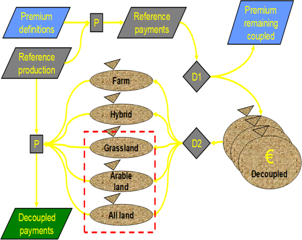
The general way these premiums are introduced in CAPRI is shown below. From a reference situation (expost statistical data) and the premiums valid at that time, it is first determined (Decision D1) how much of each existing payments in each scheme are continued to be payed as a coupled scheme, and how much is going into envelops for different types of decoupled payments (part of decision D2). That envelop can be at farm, regional or Member State level and can be implemented in different ways (e.g. historic implementation, regional, regional with different payment rates to arable or grass lands).
Figure 16: General way of SFP implementation in CAPRI
In opposite to the reforms until Agenda 2000, there are hence in most cases not longer premium rates or individual ceilings in hectares found in legal texts. Rather, these are calculated by the model itself from the decoupled part of the “old” Mac Sharry and Agenda 2000 premiums which introduces additional complexity in the model code.
Only an overall budget envelop is given covering all pillar I premiums of the EU CAP (“old” MacSharry and Agenda 2000 premiums, SPS premiums, article 63/68/69 premiums, etc.) per Member State nad per year on the position p_premDataE(MS,SIMY,“DPMTR”,“CEILVAL”) in ‘pol_input\mtr_hc.gms’. Here MS refers to member states and SIMY to a certain year.
Single area payment scheme (SAPS)
The MS who joined the EU since 2004 could choose to apply the single area payment scheme (SAPS), a simplified area payment system, for a transitory period until end 2010 or to apply the same system as in the EU-15 immediately. The most important difference between the SPS and the SAPS is that the entitlements under the SPS can be transferred between farms.
From a technical viewpoint, the single-area premium scheme (SAPS) is the easiest to implement:
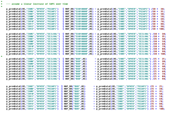
As it defines a flat rate premiums per ha of agricultural land. The ceilings in values and thus the application rates per ha are step wise increased over time:
To reach their full level in 2013 (EU 10) or 2016 (Bulgaria and Romania).
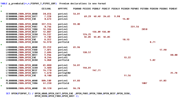
During that transition period where not yet the full EU premiums were paid out, the Member States had the right to paid up to certain limits to so-called complementary national direct payments (the list of schemes used in CAPRI was shown above). They also edited in a tabular format:
These top-ups have to be reduced towards the end of the period where the the Pillar I premiums are phased in:
Non-SAPS implementation
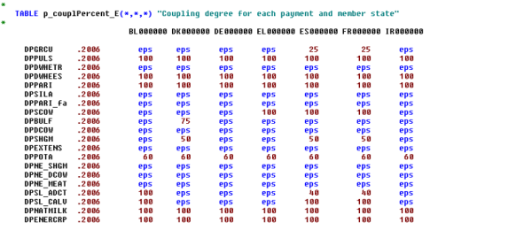
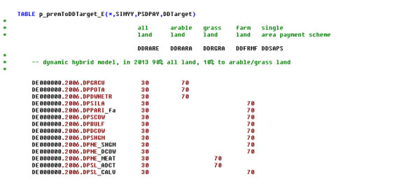
The non-SAPS implementation of the Mid-Term Review package is far more demanding. First of all, the countries could, at least in the earlier years of the reform, keep certain percentages of specific premium scheme still coupled to production. These coupling factors are stored on the parameter p_couplPercent_E:
The amount of payments which is not kept coupled is then paid out to different implementations of the MTR:
- Regional implementation where all arable crops (PGARAB)
- And permanent grass land (PGGRAS) is eligble
- The historic implementation
The exact set member ship depends on the year. The distribution shares which map the decoupled part of the premiums received under the Agenda package (see above) to these implementation schemes are edited on the Table “p_premToDDTarget_E”
That information is the basis to define regional premium envelops (= CEILVAL) for the different Member states. That is a rather complex program (‘policy\calc_mtr.gms’). A first key statement defines the remaining budget envelops for the still coupled payments. It takes the minimum of the existing ceiling values for that scheme (CEILVAL) or the total payments paid out times the modulation factors and multiplies it with the coupling degree.
There two other factors:
- A possible greening share according to the October 2011 proposal by the Commission, see the section on CAP 2014-2020 for more details
- A national ceiling cut factor which aligns the envelops calculated from the past payments with he total MTR ceiling as defined in the legal texts.
The part which is not longer coupled goes into the decoupled schemes:

The total budget for the new MTR schemes is derived from the summation of all the old Agenda premiums. The total payments under a scheme such as the Grandes Cultures schemes are corrected for any possible remaining coupled payments:
After that, a possible share going into the greening payment (from 2014) is deducted:
And, finally, a factor is applied which lines up the total historic payments as defined from the CAPRI data and premium schemes in that Member State with the total MTR envelop:
That sum if then distributed to the relevant MTR implementation scheme according to the distribution keys defined above:
These calculation require that first the total premiums received in the history period are calculated which is done in ‘policy\calc_mtr_top.gms’.
CAP 2014-2020
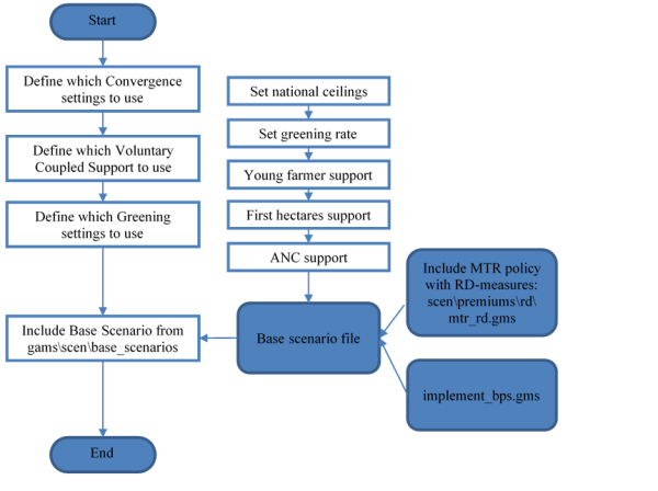
From 2014 onwards, a new agricultural policy entered into force. The key elements of the policy were (i) convergence of payment rates between member states and farmers within member states, (ii) the expansion of the option to use coupled support beyond the previous articles 68/69, and (iii) the introduction of three “greening requirements”. These elements were introduced into CAPRI, and their use can be inspected in the commonly used baseline policy file “gams\pol_input\cap_after_2014\ref.gms”, the entire content of which is shown below:
Since the mechanisms behind each of the three elements is somewhat complex, the file relies on include files to define each of the three components. The include files are stored in the scenario directory (gams\scen) of the CAPRI system, and which particular include files to use is indicated by the string variables ($setGlobal) in the first three code lines. The actual logic of the policy file, also the inclusion of the indicated three files, takes place in the file included in the final line, referred to as the base scenario file.
Convergence between member states is set by adjusting the total budget of the CAP first pillar. Regarding the convergence of payment values per entitlement (IUVs, for Individual Unit Values) inside countries, the regulation allows ample room for national customization. Countries define the regions within which convergence occurs, the end year by which convergence shall be achieved, any remaining maximum span for the IUVs after convergence, and the mathematical formula to use for reducing high IUVs and increasing low ones. The file gams\scen\premiums\bps_convergence.gms defines the options chosen by member states in 2014.
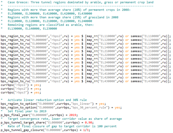
Two different uses of the convergence mechanism are illustrated by Austria and Greece, which apply very different models. Austria applies the full convergence using a linear model over time, with the same target payment rate in all of Austria. The convergence should be complete in 2019. This is obtained by assigning all Austrian regions to one generic “BPS-region”, for convenience the first one, called “rbps1”. Since the convergence mechanism later on works per member state, it is no problem that rbps1 is also used for e.g. the Netherlands. Then, the convergence option is set to “bps_linear” and the target year to 2019. Finally, the two parameters defining the rate of the final convergence are set, or, if you like, the width at the end of the convergence funnel and the handling of payments outside of that funnel. For Austria, the parameters are both set to “1”, which means that all farms will get exactly the same payments per hectare after convergence is complete in 2019.
Greece applies different models for different types of regions, depending on the character of agriculture in the region. We approximate this in CAPRI by classifying the NUTS2-regions according to the shares of arable land, grass land and permanent crops in a historical year (2008). Based on those shares, three BPS-regions are created, within each of which the same convergence model is applied. The convergence is linear, but with the additional 30-percent-rule applied, defining that no farm (supply model region) should get more than 30 percent higher payments per hectare than the average of the BPS-region. Convergence proceeds up to the year 2019, and in each year, the lower limit for convergence, expressed as a share of the averge of the BPS-region, is set to 90%. The lower limit defines whether a farm needs convergence or not. Farms above the lower limit will get the same payments per unit as before, but for farms below the limit, the final option “p_bps_tunnel_gap_closure” kicks in, and defines what share of the gap to the lower convergence limit should be closed. For Greece, this value is set to 1/3, implying that for a farm receiving less than 90% of the average payment in the BPS-region, 1/3 of the gap shall be closed. The increased premiums are financed by a linear reduction of the payments to all farms with payments above the average payment, while also capping the highest premiums to be no more than 30% higher than the regional average.
The code implementing the logic behind these various settings is generic and found in the file “gams\policy\implement_bps.gms”. The result is a payment per region, defined using the general premium mechanism of CAPRI, that is called “dp_bps” and with the eligible activity list “pgsaps”. The application type is “perLevl” and the budget is set on national level in the base scenario file “gams\scen\base_scenarios\cap_2014_2020.gms”.
Voluntary Coupled Support is defined using the standard premium mechanisms of CAPRI, based on notifications received from the European Commission. We have interpreted the notified target activities in terms of CAPRI activities, and set budget ceilings and nominal amounts in the file “gams\scen\premiums\coupling\cap_2013_2020_vcs.gms”.
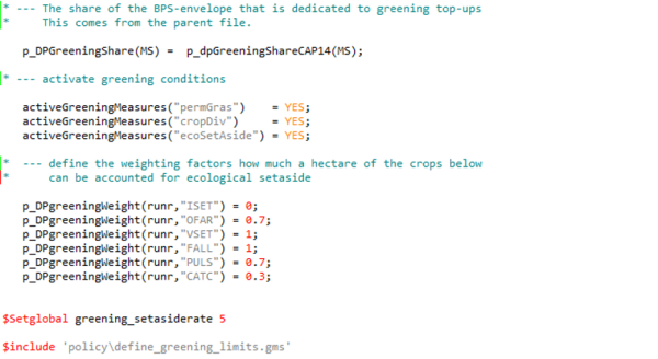
The Greening Measures can be steered by the modeller. Even though the greening in itself is complex in implementation, the choices open to the CAPRI modeller are limited. The standard greening policy switches can be inspected in the file “gams\scen\premiums\greening\cap_2013_2020_greening.gms”:
The first statement defines the share of the national pillar 1 envelope that is dedicated to the “greening top-up”. By default, this is 30%. Then, a set of active greening measures is populated. There are three options available, and by default, they are all active:
- The share of permanent grass land to arable land cannot decline relative to the base year.
- A minimum measure of crop-diversity must be maintained.
- A share of land must be allocated to certain activities counting as “ecological set-aside”.
The shares of activities eligible as ecological set-aside is then defined in the concluding parameter definition in the file. The set-aside rate itself is defined as a string variable “$setglobal greening_setasiderate 5”, defining it to be 5% by default. The three greening restrictions are implemented as constraints in the supply models. The greening top-up is implemented as a standard CAPRI premium called DPGREEN. The logic behind the greening restrictions is activated in the include file “policy\define_greening_limits.gms”.
The CAP 2014-2020 also contains three more payment schemes: Support to young farmers, support to smaller farms (first hectares) and support to areas with natural constraints (ANC). These payment schemes, with their associated budgets, are defined in the base scenario file.
The following figure summarizes the logic of the CAP 2014-2020 reference policy as implemented in the CAPRI policy module in the policy file pol_input\cap_after_2014\ref.gms.
Figure 17: The logic of the CAP 2014-2020 reference policy as implemented in the CAPRI policy module
Tradable Single Premium Scheme entitlements
With the so-called Mid Term Review of the Common Agricultural Policy, the so-called Single Farm Premium (SFP) as a decoupled payment was introduced which is implemented as a subsidy which does not require production, is subject to cross-compliance and paid per ha up to a number of entitlements. The original entitlements, defined on a hectare basis, had been distributed to farmers operating the land and not the land owners. Both land and entitlements can be traded independently from each other. After a sequence of reform steps, basically all crop production sectors are now included in the subsidy program, so that farmers can be assumed to have received entitlements for all hectares they cropped historically. The same was true from the beginning for the so-called regional implementation. If the land available to agriculture decreases, e.g. by urbanization, some entitlements cannot not longer be matched with a hectare of eligible land. Such unused entitlements are removed from the markets after a number of years.
In CAPRI, the assumption in the baseline is that all hectares used by agriculture are able to claim the SFP and that any unused entitlements had been removed so that the SFP becomes fully capitalized into land. Subsequent changes in the premiums including the SFP, prices or other policy instruments in a counterfactual run could decrease the marginal returns to agricultural land. Based on the land supply curve implemented in CAPRI, agricultural land use would shrink and some entitlements become unused. Vice versa, if changes let the marginal return to land increase, the entitlements become the limiting factor to claim the subsidy. The increase is thus mapped into an economic rent to the entitlement. If changes generate rents on entitlements in some farm types and not in others, one would assume that trade in entitlements will occur. A simple algorithm to trade the entitlement is now included in CAPRI and described below.
Switching on the entitlement trade
The trade module is implemented in the file ‘policy\prem_entl_trade.gms’ which is included on demand in capmod and called in each iteration
By default, the entitlement trade is switched OFF in the general settings file of CAPMOD, called gams\capmod\set_global_variables.gms
The basic idea of the module is very simple: shift entitlements from farm type or regions which unused entitlements to other farm types or regions which have an economic rent on their entitlements. The trading entities should receive the very same premium on the entitlement for the current implementation in the code. One should hence set the trade level according to the regional level for which flat rate premiums are implemented as shown below in an example:
How the entitlement trade works
The following code pieces are taken from ‘policy\prem_entl_trade.gms’. In a first step, the demand of entitlements is determined. The dual value does only provide an indication that entitlements are scarce, but not how many additional entitlements are needed. Accordingly, first, the average marginal value of the different type of entitlements is determined:
From these a maximum of 10% is defined as the demand in each iteration:
In order to take differences in the marginal returns into account, an indicator based on the squared value is used:
It serves as the distribution key of unused entitlements, which are determined as follows:
Next, the number of unused entitlements is stored:
As seen, only 50% of the unused entitlements are released in any iteration. We next determine the size of the markets, i.e. total demand and supply:
The supply is then distributed according to the squared value of the individual demanders
An example printout
The following code snippet shows an example for a NUTS2 regions and the related farm types for a test run for Greece without the market module:
As seen from above, we have two farm types in the starting situation which acts as demanders, i.e. have a marginal value on their entitlements (016 and 999). Their marginal value on the entitlement is quite high in the starting situation with > 125 € / entitlement. We have also a total of 3639 ha after the first round of unused entitlements which can be sold to the demanders. Distributing half of them (ca. 1800 ha) to the two demanders reduces the marginal value of the entitlements already below 95€, the next round distributed ca. 900 ha and brings the price down to 50€ until in the last round almost nothing is left for distribution and the value of the entitlements has dropped below 10€. The reader should note the trade is not yet taking into account in the income calculation of the farm types.
Finally, we come to the main point which motivated the introduction of that module. As indicated above, we interpret the SFP as a subsidy to agricultural land use which at the margin is capitalized in the land rent. It thus increases the marginal returns to land use in agriculture. In our baseline, we start with a situation with an assumed equilibrium in land markets, i.e. marginal returns in agriculture including any subsidies are equal to marginal returns of alternative uses.
Reducing the SFP will render agricultural land use less competitive so that land owner will rent out less to agriculture and put the land into other uses. That effect can be clearly seen below in the first iteration: in the farm types where the SFP drops due to uniform SFP at NUTS2 in Greece, land use is reduced. Total land use in Greece drops by 1.2%. But if we re-distribute the subsidy between farm types, farms which were competing before with below average subsidies against alternative land use possibilities now would like to expand land use. Without additional entitlements, they cannot: the marginal return on the next ha drops by the SFP rate. But once they buy entitlements, they offset a larger part of the land loss: in step twp, the reduction is only about 0.6%. And towards the end, the basically a no-change in land use, as we would have assumed at the aggregated level if the same type of subsidy is paid on average with the same rate.
Pillar II
Overview
Modelling of Pillar II for an EU-wide assessment provides a specific challenge given data availability regarding measures which are programmed and implemented at Member State or even regional level. Official reporting of measures under Pillar II in standardized data bases uses a rather rough categorisation, so are e.g. all agri-environmental measures grouped into one category. But even at that rather aggregated level, there is no ready to use data base available to researchers, especially with a regional resolution. A first task therefore consisted in building up a suitable data base on funds for Rural Development measures, a task undertaken by a team which had already compiled such data in the past (BALDOCK et.al. 2002).
The most important measures from a budgetary view point are the Agri-Environmental Schemes and the Less Favourite Area Payments. Therefore some care must be taken to model these measures accurately. The project draws here on the work of a study by LEI and IEEP (LEI and IEEP 2009) for DG-AGRI, which use in the case of the agri-environmental payments analysis based on FADN and for LFA based on FADN and CLUE (Verburg et.al. 2010) results.
Table 26: Overview of pillar II measures modelled in CAPRI
| Measure type | Measure codes EU | Modelling approach in CAPRI |
| LFAs | 211-212 | Regional direct support. Distribution over sectors and regions based on FADN data and CLUE results. |
| Natura 2000 | 213,224 | Regional direct support. Distribution over sectors and regions based on FADN data and CLUE results. Conditional on extensive technology being used. |
| Agri-environment | 214-215 | Regional direct support. Distribution over sectors and regions based on FADN data. 50% of the support directed towards TF8 farm types 1, 2, 3, 4 and 8 is conditional on extensive technology being used, for remaining amounts extensive as well as intensive technology is eligible. |
Modelling of LFA
The LFA measure was implemented as a direct payment to cropping and grassland, with the same amount for all cropping activities except for fallow land. The first challenge encountered when implementing the LFA premiums is that the regions do not coincide with the administrative regions used in CAPRI. – Recall that CAPRI only has one single representative firm in each nuts 2 region (or up to nine farm types). In reality, thus, only a share, generally much less than 100%, of the land in a nuts region is eligible for LFA payments, and it may very well be the case that the agricultural production on that land is different from the regional average. For example, one may expect that a mountainous LFA area contains more grass land than the surrounding flat land agricultural areas in the same nuts 2 region. In order to capture a possible bias of this nature, a GIS tool (CLUE-model) was used to compute the shares \(S_{ij}\) of LFA in different broad land use classes j \(\in\) {non-irrigated arable land, irrigated arable land, pasture, permanent crops} in each region i. Those shares were used to compute a (potentially) different nominal premium amount for crops belonging to each class j. The so computed different amounts were taken to reflect the biased distribution of crops inside and outside of LFA regions. Since CLUE does not distinguish “Mountainous” and “Other” LFA, the nominal amount A to which the shares S were applied was assumed the same everywhere: 250 euro, the maximum amount in mountainous LFA regions.
\begin{equation} P_{ij} =AS_{ij} \end{equation}
where
P = Premium per hectare
i = Region
j = Group of crops
A = Maximum amount per hectare, 250 euro
S = Share of LFA in all land of class j
A value ceiling for the premium was computed by adding the budgets for the component measures. Recall that the premium module of CAPRI will apply a cut factor to the amount P such that the ceiling is not overshot.
In economic terms, the potentially different premium rates for different groups of crops has a production effect, so that the type of production in CAPRI that receives the higher rates may expand on the expense of other activities. The interpretation would be that more farmers in the LFA areas comply with the LFA eligibility rules and modify their production plans to comply with the criteria there. Nevertheless, this is a simplification, because in CAPRI, no special technical restrictions are required in order to comply with the payment.
Modelling of N2k
Each production activity in CAPRI is split into a low and high yield variant with adjusted input coefficients, and thus own costs and revenues, such that their weighted average recovers regional resp. farm type means. The N2k premiums are modelled in pretty much the same way as the LFA premiums, but now with the additional assumption that the payments are conditional on extensification. This was implemented using the two alternative technologies. Thus, only the technological alternative with yield 20% below nuts2 average and lower input requirements (following a yield function) was made eligible for the payment. This is based on no empirical investigation, but is a pure assumption based on the frequently stated fact that the N2k payments are conditional on extensive management practices.
The interpretation is the following: If more money is spent on the measure, more farmers within the designated areas may switch to extensive agriculture. Then the average payment per hectare of the nuts 2 region would increase, reflecting that a larger share of the farmers now participate in the measure. It is today indeed the case that not all farms within an N2k area receive support.
Modelling agri-environmental payments
The agri-environmental payments is a very diverse set of measures, which accounts for the largest share of the second pillar. In the modelling approach opted for here, with one aggregated measure “05 agri-environment”, a uniform implementation across member states cannot be used, which is in contrast to the LFA and N2k measures. Instead, a way of capturing the national or even regional preferences within the agri-environmental schemes must be sought.
The method for “nationalization” of the AE scheme employed here is to use the distribution of the sum of the AE measures, i.e. the measure allocated to class 05, to agricultural sectors using the receipts by farm types according to FADN in 2005 as key. This implies linking the support to production. Whether this corresponds to reality is an empirical question. It is doubtless the case for some measures in some regions, but certainly not so for all AE measures in all regions. Refining the implementation would thus involve conditioning the support on technical constraints. Nevertheless, the implementation described above has the merit that it allocates the correct budget, resulting from the LEI budget model, to approximately the right group of farmers.
Table 27: Mapping from aggregated farm types in FADN (TF8) to activity groups in CAPRI
| TF8 type | Group of activities in CAPRI |
| 1 | Grandes Cultures |
| 2 | Vegetables |
| 3 | Wine |
| 4 | Permanent crops |
| 5 | Dairy cows including pastures |
| 6 | Suckler cows, sheep and goats, including pastures |
| 7 | Pigs and poultry |
| 8 | All agricultural activities |
The agri-environmental (AE) payments are implemented as extensification subsidies, and they are distributed to regions based on the distribution of less-favoured areas across regions. However, the distribution is modulated by the national level shares of farms in or out of LFA receiving AE support. We needed the following two probabilities:
p_landPartition(ru,lcAgri,”LFA”): The share of land of each land class that is LFA (computed based on extrations from the DYNA-CLUE database).
p_aeLfa(ms,tf8): The probability of a farm of type tf8 having agri-environmental support conditional on the farm being in an LFA region or not, computed based on the FADN sample.
Then, the payment rate for each region is set in proportion to the weighted share of farms likely to have some AE support, predicted by the regional share of each land class (grass, arable) being classified as LFA in each region times the share of farms in/out of LFA having AE-support in the national FADN sample. The computation takes place in policy\rd_logic.gms:
Note that the code does not know how high the absolute level of payments shall be for each region, but allocates the relative levels. Then, the national ceiling for AE payments are applied to adjust all regional payments until the ceiling is respected.
Finally, an extensification effect to the AE payments is introduced using the possibility to make technological variants differently eligible.
Co-financing rates, assignment of premiums to pillars, WTO boxes and PSE-types
EU and national budget contribution
The reporting part of the system was expanded to account for (co-)financing rates of the different schemes, so that contributions from EU and national budgets can be differentiated. The underlying factors are currently defined in ‘policy\policy_sets.gms’:
PSEs
The mapping to the PSE-types is defined in ‘policy\policy_sets.gms’:
WTO boxes
In a similar fashion, the premiums are allocated to the WTO boxes. The following payments are allocated to the green box (‘policy\policy_sets.gms’):
The blue box, i.e.g payments under supply control or only paid up to certain upper limits, is defined as along with remaining amber box payments in Norway:
Currently, the following budget categories are supported (see ‘sets.gms’ and ‘policy\policy_sets.gms’):
In ‘reports\feoga.gms’, these categories are first aggregated for each activities from actual schemes (“PRME” = actual payment rate, p_budToPsdpay: distribution key):
In order to come to a product based accounting scheme as used by the PSEs and WTO, these payments are assigned to the main outputs of the activities. Payments to obligatory set-aside are allocated to the activities according to set-aside rates:
For a discussion about the WTO and PSE Boxes and their implementation in CAPRI see: Mittenzwei, K., Britz, W. und Wieck, C. (2012): Studying the effects of domestic support provisions on global agricultural trade: WTO and OECD policy indicators in the CAPRI model, selected paper presented at the 15th Annual Conference on Global Economic Analysis, “New Challenges for Global Trade and Sustainable Development”, June 27-29,2012, Geneva (Switzerland).

