Table of Contents
Dual analysis (T. Jansson)
Constrained optimisation background
The supply model in CAPRI is a constrained optimization problem, maximizing profits plus a nonlinear term subject to multiple constraints. In some simulations, production activities in the model are affected in several ways simultaneously, and it is difficult to understand what the key drivers are behind a specific change. There may be changes both in parameters of the model such as prices or subsidies and also of dual values of resources such as land or fodder. Then a dual analysis can help you decompose the impacts by explaining how much the profitability of a production activity changed due to various factors. The key idea is to analyse how each term of the first order conditions changed.
For any well-behaved optimization model (one that e.g. maximizes a concave objective function on a convex constraint set) we can formulate the first order condition stating that in the optimal point, the sum of all marginal changes of all variables would provoke no change1) in the objective function. Let \(i=1…n\) be activities in the model, \(x_i\) be the level of activity i, \( f:\mathbb{R} _n\rightarrow \mathbb{R}\) be the concave and continuously differentiable objective function (e.g. profits), and \( g_j:\mathbb{R} _n\rightarrow \mathbb{R}\) be a function serving as a restriction for each of \(j=1…m\) resources. Finally, assume that all activity levels have to be non-negative2). The agent of the model acts as if solving the following maximization problem:
\begin{equation*} max \, f (x_1,...,x_n) \end{equation*}
Subject to
\begin{align} \begin{split} \begin{matrix} g_j(x_1,...,x_n) = 0 & [\lambda_j] & \forall j= 1 ... m \\ x_1 \ge 0 & [\pi_i] & \forall i= 1 ... n \end{matrix} \end{split} \end{align}
Greek letters (λ and π) in square brackets denote the Lagrange multipliers associated with each constraint. The Lagrange function3) for this problem can be written
\begin{equation} L(x_1, ... ,x_n,\lambda_1, ... , \lambda_m,\pi_1, ... , \pi_n) = f(x_1, ... ,x_n) - \sum_j \lambda_j g_j(x_1, ... ,x_n) + \sum_i\pi_ix_i \end{equation}
The necessary conditions for an optimal solution include the first order derivative of the Lagrangean with respect to the activity levels:
\begin{equation} \frac{\partial L}{\partial x_i} = \frac{\partial f}{\partial x_i} - \sum_j \lambda_j \frac{\partial g_j}{\partial x_i} + \pi_i = 0 \end{equation}
The functions f and g depend on some parameters, e.g. prices and technical i/o coefficients respectively that were not shown in the exposition above in order to reduce the size of the expressions. By changing such parameters, we introduce shocks to the model. Assume that in a reference scenario, we have prices \(p^0\) and technology \(a^0\) resulting in the solution \( (x_1^0,…,x_n^0,λ_1^0,…,λ_m^0,π_1^0,…,π_n^0 ) \). In another simulation, we have other prices \(p^*\) and technology \(a^*\) resulting in the alternative solution \( (x_1^*,…,x_n^*,λ_1^*,…,λ_m^*,π_1^*,…,π_n^* )\).
In this simulation we now would like to know more about why some particular activity \(x_i\) reacts as it does, i.e. why \(x_i^*\) is different from \(x_i^0\). We then compute each term in the first order conditions, and compare the two simulation. To be slightly more explicit, we can assume that the resources are j={“land” ,“fodder” ,“young animals” }. We can then do a comparison such as the following:

If we would compute the difference between the two rows above for each corresponding term, the differences would also sum up to zero, and each difference would mean something and have a numerical value: The first term is the change in marginal profits, the second term is the change in marginal cost of land, the third is the marginal cost of fodder, the fourth the marginal cost of young animals, and the final term the possible marginal value of a lower bound on the activity at hand. This can usually be directly translated into a storyline, like “The price increase increases the marginal profit of barley production by q euro per hectare, which leads to an expansion of production until it is matched by a similarly large increase in land rents”.
Of course, each partial derivative may be further decomposed into its smallest parts. For instance, profits may contain several items such as revenues, costs and behavioural terms.
Example – removing greening payments and requirements
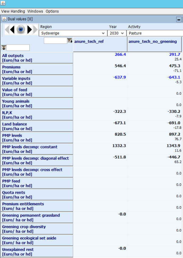
The dual analysis of the supply models is computed by a file called “supply\margcr.gms” (where margcr probably means “MARGinal Cost and Revenues”), which is always included after the last iteration. The figures below show the CAPRI GUI comparing the results of two scenarios: one reference continuing CAP after 2014 up to 2030, and a counterfactual where the greening payments and requirements are removed. We look at the results of a single region “Sydsverige” to avoid aggregation issues.
In Figure 39, we can look for the biggest changes (absolute difference between simulations is printed in brackets in the right hand column), and find a 71 euro reduction in payments. This is in line with the scenario, which removed 30% of the farm payment. All other positions adjust to some extent, and as usual with CAPRI, we find a similarly sized change in “PMP terms” (+77 euro income or reduction in costs), i.e. the behavioural terms adjust. As a note, we see that for this region, grassland is highly unprofitable in the reference scenario, and therefore the PMP term is calibrated to become a marginal income. The PMP effect is decomposed 4)into a change in the constant term (brought about by a shift between GRAI and GRAE), diagonal terms (the main effect, 65 euro) and cross effects (zero in this case).
Figure 38: Dual analysis of changes in pasture area (intensive and extensive) in a scenario removing the CAP greening components

Source: CAPRI modelling system
There are more adjustments. Also land rents drop by 18 euro, the output of grass shown in the first line increases in value by 25 euro. Both variable costs and the value of the fertilizer restriction decrease, but those effects are comparatively minor.
