module_for_agricultural_supply_at_regional_level
Table of Contents
Module for agricultural supply at regional level
Basic interactions between activities in the supply model
There are two sources for interactions between activities in simulation experiments: the objective function and constraints. In the current version of CAPRI, the objective function does solve inter-activity terms for groups of arable crops, so that the major interplay is due to constraints. The interaction is best understood by looking at the first order conditions of a programming model including PMP terms:
\begin{equation} Rev_j = Cost_j+ac_j+\sum_k bc_{j,k}Levl_k+\sum_i^m\lambda_ia_{ij} \end{equation}
The left hand side (Rev) shows the marginal revenues, which are typically equal to the fixed prices times the fixed yields plus premiums. The right hand side shows the different elements of the marginal costs. Firstly, the variable or accounting costs (Cost) which are fix as they are based on the Leontief assumption. The term \( (ac_j+\sum_k bc_{j,k}Levl_k) \) shows the marginal non-linear costs, which are increasing with the activity levels. The cross effects are only introduced to let major arable crop groups interact, whereas for fruits & vegetables, permanent crops, grassland and the animal sectors, only diagonal terms are introduced. The methodology for the estimation of these terms is described in Jansson and Heckelei (2011).
The remaining term \( (\sum_i^m\lambda_ia_{ij}) \) captures the marginal costs linked to the use of exhausted resources and is equal to the sum of the shadow prices \lambda multiplied the per unit demand of resource i for activity j; the matrix A being again based on Leontief technology. The shadow values of binding resources hence are the drivers linking the activities.
The land balance plays a central role in the CAPRI supply model. The land shadow price appears as a cost in all crop activities including fodder producing ones, so that animals are indirectly affected as well. The second major link is the availability of not-marketable feeding stuff, and finally, less important, organic fertiliser.
The basic effects are best discussed with a simple example. Assume an increase of a per hectare premium for soft wheat, all other things unchanged.
- What will happen in the model? The increased premium will lead to an imbalance between marginal revenues (= yield times prices plus premium) and marginal costs (=accounting costs, ‘resource use cost’, non-linear costs). In order to close the gap, as marginal revenues are fixed, the area under soft wheat will be increased until marginal costs of producing soft wheat have increased to a point where they are again equal to marginal revenues. As the marginal costs linked to the non-linear cost function \( (ac_j+\sum_k bc_{j,k}Levl_k) \) are increasing in activity levels, increasing the area under soft wheat will hence reduce that gap. At the same time, as the land balance must be kept closed, other crop activities must be reduced. The non-linear cost function will for these crops now provoke a countervailing effect: reducing the activity levels of competing crops will lead to lower costs for these crops. With marginal revenues (Rev) and accounting costs (Cost) fixed, that will require the shadow price of the land balance to increase.
- What will be the impact on animal activities? Again, the shadow price of the land balance will be crucial. For activities producing non-marketable feed, marginal revenues are not defined as prices times yields, but as internal feed value times prices. The internal feed value is determined as the substitution value of non-marketable fodder against other feeding stuff, and depends on their nutrient content and further feed restrictions. Increasing the shadow price of land will hence either require decreasing other costs in producing fodder or increasing the internal marginal revenues. In other words, a high shadow price of land renders non-marketable fodder less competitive compared to other feeding stuff. As feed costs are – however very slightly – increasing in quantities fed per head, feed costs for animals will increase. But as there are several requirement constraints involved, some feeding stuff may increase and other decrease. Clearly, the higher the share of non-marketable fodder in the mix for a certain animal type, the higher the effect. As marginal feed costs will increase, and marginal revenues for the animal process are not changing, other marginal costs in animal production need to be reduced, and again the non-linear cost function will be the crucial part, as the marginal cost related to it will decrease if herd sizes drop.
To summarize the supply response, increasing premiums for a crop will hence increase the cropping share of that crop, reduce the share of other crops, increase the shadow price of land, lead to less fodder production, higher fodder costs and thus reduced herd size of animals.
- What will be the impacts covered by the market? The changes in hectares will lead to increased supply of the crop with the higher premium and less supply of all other crops at given prices, i.e. one upward and many downward shifts of the supply curves. Equally, supply curves for animal products will shift downwards. On the other hand, some feed demand curve will shift as well, some upward, other downward. These shifts will move the market module away from the former fixed points where market balances were closed. For the crop product with the increased premiums, increased supply plus some changes in feed will most probably lead to lower prices, whereas prices of other crops will most probably increase. That will require new adjustments during the next iteration where the supply models are solved, with to a certain extent countervailing effects.
Table 25: Overview on a regional aggregate programming model
| Crop Activities | Animal Activities | Feed Use | Net Trade | Constraints | |
| Objective function | + Premium – Acc.Costs – variable cost function terms | + Premium – Acc.Costs – variable cost function terms | - variable cost function terms for feeding | + Price | |
| Output | + | + | - | - | = 0 |
| Area | - | < = land supply | |||
| Set aside | +/- | = 0 | |||
| Quotas | - | - | < = Ref. Quantity | ||
| Fertilizer needs | - | + | + | = 0 | |
| Feed requirements | - | + | + | = 0 |
Detailed discussion of the equations in the supply model
The definition of the supply model can be found in ‘supply\supply_model.gms’
Feed block
The feed block ensures that the requirements of the animal processes in terms of feed energy and protein are met and links these to the markets and crop production decisions.
\begin{equation} \overline{AREQ}_{r,act,req} \overline{DAYS}_{r,act,req}= \sum_{feed} FEDNG_{r,act,feed} \overline{REQCNT}_{r,act,feed} \end{equation}
The left hand side captures the daily animal requirements (AREQ) for each region r, animal activity act and requirement AREQ multiplied with the days (DAYS) the animal is in the production process. Both are parameters fixed during the solution of the modelling system. The right hand side ensures that the requirement content of the actual feed mix represented by the feeding (FEDNG) of certain type of feed to the animals multiplied with the requirement content (REQCNT) in the regions covers these nutritional demands. Requirements and contents are specified in the feed calibration while production days are determined in the “COCO1” module. Total feed use (FEDUSE) in a region is defined as the feeding per head multiplied with the activity level (LEVL) for the animal activities:
\begin{equation} FEDUSE_{r,feed} = \sum_{aact} LEVL_{r,aact} FEDNG_{r,aact,feed} \end{equation}
Total feed use might be either produced regionally in the case of fodder assumed not tradable (grass, fodder root crops, silage maize, other fodder from arable land), or bought from the market at fixed prices.
Land balances and set-aside restrictions
The model distinguishes arable and grassland and comprises thus two land balances:
\begin{equation} \overline{LEVL}_{r,"arab"} \le \sum_{arab} LEVL_{r,arab} \end{equation}
\begin{equation} \overline{LEVL}_{r,"gras"} \le LEVL_{r,"grae"} + LEVL_{r,"grai"} \end{equation}
Both land balances might become slack if marginal returns to land drops to zero. For arable land, idling land not in set-aside (activity FALL) is a further explicit activity. For the grassland, the model distinguishes two types with different yields (GRAE: grassland extensive, GRAI: grassland intensive) so that idling grassland can be expressed of an average lower production intensity of grassland by changing the mix between the two intensities.
The model comprises a land use module with two major components:
- Imperfect substitution between arable and grass lands depending on returns to the two types of agricultural land uses.
- A land supply curve which determines the land available to agriculture as a function to the returns to land.
There are hence two further equations:
\begin{equation} \overline{LEVL}_{r,"uaar"} = \overline{LEVL}_{r,"arab"} +\overline{LEVL}_{r,"gras"} \end{equation}
And a further one which prevents numerical problems with the terms relating to land supply in the objective function
\begin{equation} \overline{LEVL}_{r,"uaar"} = 0.999 \overline{LEVL}_{r,"asym"} \end{equation}
Where “asym” is the land asymptote, i.e. the maximal amount of economically usable agricultural area in a region when the agricultural land rent goes towards infinity. For an application where the land market is used see Renwick et al. (2013).
Set aside policies have changed frequently during CAP reforms. The recent specification is covered in the context of the premium modelling in Section Premium module. The obligatory set-aside restriction introduced by the McSharry reform 1992 and valid until the implementation of the Luxembourg compromise of June 2003 has been explicitly modelled through this equation:
\begin{align} \begin{split} &LEVL_{r,"iset"} + LEVL_{r,"gset"} + LEVL_{r,"tset"} \\ &=\sum_{arab} LEVL_{r,arab}\left(1-NONS_{r,arab}\right ) \frac {1/100SETR_{r,arab}}{1- 1/100 SETR_{r,arab}} \end{split} \end{align}
LEVL_{r,“iset”}As seen from above, the model distinguishes between three types of obligatory set-aside: idling (ISET), for grass land use (GSET) and for forestation purposes (TSET). The share of so-called non-food production exempt from set-aside (NONS) for each activity and region is fixed and given.
The equation above is replaced for years where the Luxembourg compromise of June 2003 is implemented by a Member State, where the level of obligatory set-aside is fixed instead to the historical obligations.
For certain years of the McSharry reform, the total share of set-aside – be it obligatory or voluntary – on a list of certain crops was not allowed to exceed a certain ceiling. That restriction is captured by the following equation:
\begin{align} \begin{split} &LEVL_{r,"iset"} + LEVL_{r,"gset"} + LEVL_{r,"tset"}+ LEVL_{r,"vset"} \\ & \le \sum_{arab \wedge SETF_{r,arab}} LEVL_{r,arab}/\overline{MXSETA} \end{split} \end{align}
Fertilising block
As of CAPRI Stable Release 2.1, the fertilizer allocation was modified, and this section of the documentation updated. Notation has changed compared with previous versions of the model and documentation. Here, we represent the equations in more general mathematical notation, avoiding the long GAMS code names of the source code, in order to save space.
We distinguish the three macro-nutrients N, P and K. The supply and uptake of those nutrients are modelled in a uniform way, save for the fact that there is fixation and atmospheric deposition only of N.
Each crop has a requirement per hectare, calculated based on the yield. Yields are exogenous from the vantage point of the producer, but there are alternative technologies available for each cropping activity, and a separable, i.e. handled outside of the optimization model, relation between prices and optimal yields.
From the basic nutrient requirement we first deduct the rate of biological fixation (only for nitrogen and selected crops). The remainder is inflated by a (calibrated) factor and additive term of over-fertilization, and then scaled with a soil-specific factor (only for nitrogen), to arrive at the total amount of nutrients that need to be supplied to the crop. This is the left hand side of Equation 96  .
.
Nutrient supply, shown on the right handside, comes from mineral fertilizer, manure, crop residues and atmospheric deposition. Mineral fertilizer may have ammonia losses during application. For manure, there are both losses and inefficiencies. When manure is applied to crops, there is an efficiency factor applied to the nutrient content (denoted by ϕ_(r,“excr”, n) ), corresponding to the Fertilizer Value (FV) of manure relative to mineral fertilizer. The efficiency factor is a key parameter of interest in simulations carried out in some studies. Crop residues can be re-distributed among crop groups for annual arable crops but not for grassland and permanent crops, where it stays with the crop that produced it. For crop residues there is both a loss rate and a fertilizer value.
\begin{align}
\begin{split}
&\sum_{i \in I \, j,k} \left[ levl_{rik} \left ( ret_{rni} (1-biofix_{rni}) \lambda_{rnik}^{prop} + \lambda_{rni}^{const} \right ) soil_{rn} \, yf_{rnik} \right ] \\
& = fmine_{rni}(1-loss_{rn}) +fexcr_{rni} \phi_{r,excr,n} +(1-isPerm_j)fcres_{rni}(1-loss_{rn})\phi_{r,cres,n}\\
& + isPerm_j \sum_{ i \in I \, j,k} levl_{rik}res_{rni}(techf_{rink}+1)(1-loss_{rn})\phi_r,cres,n \\
& \forall r,n,j
\end{split}
\end{align}
Indices:
\(r\) = region
\(i\) = crop
\(j\) = crop group
\(k\) = technological crop option (high/low yield)
\(n\) = nutrient (N/P/K)
\(isPerm_j\) = indicates that crop group \(j\) contains permanent crops
Endogenous choice variables:
\(levl_{rik}\) = Area (ha) of each crop \(i\) and technology \(k\) in region \(r\).
\(fmine_{rnj}\) = Application of mineral fertilizer \(n\) to crop group \(j\) in region \(r\).
\(fexcr_{rnj}\) = Application of manure \(n\) to crop group \(j\) in region \(r\).
\(fcrex_{rnj}\) = Allocation of crop residue \(n\) to crop group \(j\) in region \(r\).
Parameters:
\(ret_{rni}\) = Retention (uptake) of nutrients by the crop
\(res_{rni}\) = Crop residues output
\(biofix_{rni}\) = Biological fixation, share (only for N and selected crops)
\(λ_{rnik}^{prop} \) = Over-fertilization factor, calibrated
\(λ_{rni}^{const} \) = Over-fertilization term, calibrated
\(soil_{rn}\) = Soil factor
\(yf_{rnik}\) = Yield factor for technologies
\(loss_{rn}\) = Loss rate
\(ϕ_{r",excr" ,n}\) = Nutrient availability ratio for manure
\(ϕ_{r,"cres" ,n}\) = Nutrient availability ratio for crop residues
The reader may have noted that there is no loss rate for manure in the Equation 96 . CAPRI does contain such loss rates, but they are specific for each animal type and therefore happens on the manure supply side of the regional manure balance (see section on input allocation).
The model contains three types of manure: N-manure, P-manure and K-manure. From an agricultural point of view this may seem odd. It might be more intuitive to think of one type of manure per animal category. The motivation is to keep the system simple and flexible. With the present representation, where each animal category supplies N, P, and K-manure, the number of manure classes can be limited and yet the unique mix of nutrients from each animal category can be defined.
The supply of each manure type is collected in a “pool” for each regional farm model, i.e. for each NUTS2 region. Regions within a member state may trade manure, subject to a cost. The supply in the pool plus the traded quantities has to be distributed to the crops in the region, i.e. there is an equality-restriction in place. This is handled in the equations “FertDistExcr_” and “ManureNPK_”. Note that fertilizer flows are measured in tons, for the sake of scaling, whereas other total quantities in CAPRI are measured in 1000 tons. Hence the factors 1000 and 0.001.
\begin{equation} \sum_j fexcr_{rnj}= 1000 v\_ManureNPK_{rn} \end{equation}
\begin{equation} v\_ManureNPK_{rn} + \sum_s T_{rs}nutshr_{rn} = 0.001 \sum_{i\in Anim_j,k} levl_{rik}o_{rnik}(1-loss_{rin}) \quad \forall r, n \end{equation}
where
\(o_{rnik}\) is the output of manure nutrient \(n\) from animal type \(i\) using technology \(k\) in region \(r\),
\(nutshr_{rn}\) is the average content of each nutrient in the regional manure pool,
\(T_{rs}\) is the quantity of manure traded from \(r\) to \(s\),
\(isAnim_{i}\) indicates that activity \(i\) is an animal production activity
Equation “FertDistMine_” allocates total mineral fertilizer sales to the crops / group of crops.
\begin{equation} \sum_j fmine_{rnj} = -netPutQuant_{rn} \end{equation}
Finally, crop residues and atmospheric definition are distributed in equation “FertDistCres_”.
\begin{equation} \sum_j fcers_{rnj} = \sum_{i \notin isPerm_j,k} levl_{rik}res_{rni}(techf_{rink}+1) \end{equation}
One flow from a source s={“mine” ,“cres” ,“excr” } to a sink j={“crop groups”} can in general be anything from zero and upwards. The nutrient balance equations above do not uniquely determine each flow of nutrients from sources to sinks, but it is indeed possible that in one simulation, say, a particular crop group gets much crop residues and little manure, whereas the opposite holds in the next simulation. The total balances will hold equally well in either situation, and the profits will not be affected since the same total amount of mineral fertilizer is purchased, but we do have a stability problem for the model. Furthermore, the different nutrient flows may influence the greenhouse gas emission coefficients of crops (if e.g. the emissions of enteric fermentation follows the manure to the crops). The problem is under-determined, or ill-posed.
To resolve the ill-posedness of the fertilizer distribution, we propose a probabilistic approach. This means that we do not introduce any additional economic model for the allocation that somehow makes increasing fertilizer flows more expensive. Instead, we assume that whatever the reasons the farmers have for choosing a particular distribution, those reasons are similar in two simulations, and therefore the fertilizer flows are also similar. Thus, a larger deviation from some reference flows is deemed improbable, albeit not costlier than the situation with the reference flows.
To develop this probabilistic model, we assume that the decisions of the farmer are separable and taken in two steps: first, the farmer decides about the cropping plan and just ensures that the total amount of fertilizer available is sufficient. This is called the outer model. Then, a statistical model is solved that finds the most probable fertilizer flows out of the continuum of possible ones. This is called the inner model. The structure with outer and inner models makes the problem a bi-level programming one.
To implement the bi-level programming problem in a way that does not change the present structure of the model (with just one optimization solve of the representative farm model) we implement the inner model by its optimality conditions. By carefully choosing the proper probability density functions we ensure that no complementary slackness conditions are needed, so that the inner model is simple to solve. For this the gamma density function is very suitable, as it has a support from zero to infinity, with a probability that goes towards zero as the random variable goes to zero.
The parameters of the gamma function are determined in the calibration step, described further below, and then kept constant in simulation. The gamma density function for some random variable x has the form
\begin{equation} p(x|\alpha,\beta) = \frac {\beta^{\alpha}}{\Gamma(\alpha)}x^{\alpha-1}e^{-\beta x} \end{equation}
where Γ(α) is the gamma function, and α and β are parameters that determine the shape of the density function. The gamma density is nonlinear, and the joint density, being the product of the densities of all nutrient flows, is even more so. In order to reduce nonlinearity we note that are interested in finding the highest posterior density, i.e. maximizing a joint density function, and since the maximum is invariant to monotonous positive transformations we compute the logarithm of the joint density, which will be the sum of terms like the following (the constant term has been omitted since it also does not influence the optimal solution for x):
\begin{equation} log \, p(x|\alpha,\beta) \propto (\alpha-1)log \, x-\beta x \end{equation}
Maximization of the logged density under the constraints that the nutrient balance restrictions of the supply modes have to be met gives a set of equations that define explicit and unique fertilizer flows, where v are the Lagrange multipliers of the source-pool restrictions and u the Lagrange multipliers of the nutrient balance equation.
\begin{equation} \text{FOC w.r.t. manure use:} \\ \frac {\alpha_{r,excr,nj}-1}{fexcr_{rnj}} - \beta_{r,excr,nj} - v_{r,excr,n}+\phi_{r,excr,n}u_{rnj} = 0 \end{equation}
\begin{equation} \text{FOC w.r.t. crop residues use:} \\ \frac {\alpha_{r,cres,nj}-1}{fcres_{rnj}} - \beta_{r,cres,nj} - v_{r,cres,n}+(1-loss_{rn}\phi_{r,excr,n}u_{rnj} = 0 \forall j\notin isPerm_j \end{equation}
\begin{equation} \text{FOC w.r.t. mineral feritilzer use:} \\ \frac {\alpha_{r,mine,nj}-1}{fmine_{rnj}} - \beta_{r,mine,nj} - v_{r,mine,n}+(1-loss_{rn}u_{rnj} = 0 \end{equation}
The system of FOC contains expressions of the type \(1/fmine\) which is likely to impair performance as the second derivatives are not constant (CONOPT computes second derivatives). Therefore, the first term in each FOC was turned into a new variable \(z\) defined as \( z_{r,"excr" ,nj}fexcr_{r,"excr" ,nj}=\alpha_{r,"excr" ,nj}-1\), and similar for each source, which is a quadratic expression.
Balancing equations for outputs
Outputs produced must be sold – if they are tradable across regions – or used internally, as in the case of young animals or feed.
\begin{equation} \sum_{act}Levl_{r,act}OUTP_{r,act,o}=NETTRD_r^{o\notin fodder}+YANUSE_r^{o\notin oyani} +FEDUSE_r^{o\in fodder} \end{equation}
In the case of quotas (milk, for sugar beet) the sales to the market may be bounded (noting that NETTRD = v_netPutQuant in the code):

As described in the data base chapter, the concept of the EAA requires a distinction between young animals as inputs and outputs, where only the net trade is valued in the EAA on the output side. Consequently, the remonte expressed as demand for young animals on the input side must be mapped into equivalent ‘net import’ of young animals on the output side:
\begin{equation} \sum_{aact}Levl_{r,aact}I_{r,aact,yani}=YANUSE_r^{oyani \leftrightarrow iyani} \end{equation}
In combination with the standard balancing equation shown above, the NETTRD variable for young animals on the output side becomes negative if the YANUSE variable for a certain type of young animals exceeds the production inside the region.
The objective function
The objective function is split up into the linear part, the one related to the quadratic cost function for activities, and the quadratic cost function related to the feed mix costs:
\begin{equation} OBJE=\sum_r LINEAR_r+QUADRA_r+QUADRF_r \end{equation}
The linear part comprises the revenues from sales and the costs of purchases, minus the costs of allocated inputs not explicitly covered by constraints (i.e. all inputs with the exemptions of fertilisers, feed and young animals) plus premiums:
\begin{equation} LINEAR_r= \sum_{io} NETTRD_{r,io} \overline{ PRICE}_{io}+ \sum_act LEVL_{r,act}\left (\overline{PRME}_{r,act}-\overline{COST}_{r,act}\right) \end{equation}
The quadratic cost function relating to feed is defined as follows:
\begin{equation} QUDRAF_r = \sum_{aact,feed} \left[ \begin {matrix} LEVL_{r,aact}FEDNG_{r,aact,feed} \\ (a_{r,aact,feed}+ 1/2b_{r,aact,feed}FEDNG_{r,aact,feed}) \end{matrix} \right] \end{equation}
The marginal feed costs per animal increase hence linearly with an increase in the feed input coefficients per animal. It should be emphasised that this is the main mechanism that “stabilises” the feed allocation by animals. The two balances on feed energy and protein alone would otherwise leave the feed allocation indeterminate and give a rather “jumpy” simulation behaviour.
There is another more complex PMP term (equation quadra_ in supply_model.gms, not reproduced in this section) quadratic in activity levels and differentiated by the two technologies that “stabilises” the composition of activites according to previous econometric estimates or default assumptions.
A final term relates to the entitlements introduced with the 2003 Mid Term reviews. If those entitlements are overshot, a penalty term equal to the premium paid under the respective scheme (regional, historical etc.) is subtracted to the objective. Accordingly, the marginal premium for an additional ha above the entitlement ceiling is zero.
Sugar beet (M. Adenäuer, P. Witzke)
The Common Market Organisation (CMO) for sugar regulates European sugar beet supply with a system of production quotas, even after the significant reforms of 2006, up to year 2017 when the quota system expired. Before that reform, two different quotas had been established subject to different price guarantee (A and B quotas, qA and qB). Beet prices were depending on intervention prices and levies to finance the subsidised export of a part of the quota production to third countries. Sugar beets produced beyond those quotas (so called C beets) were sold as sugar on the world market at prevailing prices, i.e. formally without subsidies. However, a WTO panel initiated by Australia and Brazil concluded that the former sugar CMO involved a cross-subsidisation of C-sugar from quota sugar such that all exports of C sugar was also counted in terms of the EU’s limits on subsidised exports. As a consequence, this outlet for EU surplus production was closed. The reformed CMO therefore does not allow any exports beyond the Uruguay round limits. Instead, processing of beets to ethanol emerged as a new outlet that economically plays a similar role as former C beet production: It offers an outlet for high production quantities that exceed the quota limits of farmers, but at a reduced price. Basically, farmers face a kinked beet demand curve that potentially involved three price levels:
- A-beets receiving the highest price derived from high sugar prices (and before the 2006 reform less a small levy amount)
- B-beets receiving a lower price as the applicable levies were higher before the reform. However, the 2006 reform eliminated the distinction of A and B quotas. Furthermore, the sugar industry applied a pooling price system in many MS that also eliminated the distinction between A and B beets.
- C-beets receiving the lowest price, formerly derived from world market sugar prices, now derived from ethanol prices.
The high price sector covers for farmers at least the farm level quota endowment. However, the sugar industry may grant high prices also for a limited, “desirable” over-quota production, for example to avoid bottlenecks in sugar or ethanol production. This has been the case in some EU countries before the reform (so-called “C1 beets”) and it is also current practice (see, for example http://www.liz-online.de).
Considering a kinked demand curve and in addition yield uncertainty renders the standard profit maximisation hypothesis inappropriate for the sugar sector (at least). The CAPRI system therefore applies an expected profit maximisation framework that takes care for yield uncertainty (see Adenäuer 2005). The idea behind this is that observed C sugar productions in the past are unlikely to be an outcome of competitiveness at C beet prices rather than being the result of farmers’ aspirations to fulfil their quota rights even in case of a bad harvest. This approach essentially assumes that the “behavioural quotas” of farmers may exceed the “legal quotas” (derived from the sugar CMO) by some percentage. This percentage reflects in part the pricing behaviour of the regional sugar industry, but it may also depend on farmers expectations on the consequences of an incomplete quota fill. These aspects may be captured with the following specification of expected sugar beet revenues that substitute for the expression \(NETTRD_{r,io} \; PRICE_{io} \) (if \(io=SUGB\)) in equation below:
\begin{align} \begin{split} SegbREV_r & = p^A NETTRD_{r,SUGB} \\ & - \left( p^A-p^B\right) \left [ \begin{matrix} (1-CDFSugb(q^A))(NETTRD_{r,SUGB}-q^A) \\ + (\sigma^S)^2 PDFSugb(q^A) \end{matrix} \right] \\ & -\left(p^B-p^C\right) \left [ \begin{matrix} (1-CDFSugb(q^A+B))(NETTRD_{r,SUGB}-q^A+B) \\ + (\sigma^S)^2 PDFSugb(q^A+B) \end{matrix} \right] \end{split} \end{align}
Where \(PDFSugb_r\) and \(CDFSugb_r\) are the probability res. cumulated density functions of the NETTRD variable with the standard deviation \(\sigma^S\). \(\sigma^S\) is defined as \(NETTRD_{r,SUGB} * VCOF_r\), where the latter is the regional coefficient of yield variation estimated from FADN. \({p^ABC}\) are the prices for the three different types of sugar beet which are exogenous and linked to the EU and world market prices for sugar. The quotas \(q^A\) and \(q^{A+B}\) used in Equation 111 are the “behavioural quotas, currently specified as follows:
\begin{align} \begin{split} p^A &= legalqout^A \cdot scalefac \\ & = legalqout^A \cdot \left(\frac{NETTRD_{SUGB}^{cal}}{legalqout^A} \right )^{0.8} \end{split} \end{align}
The scaling factor to map from the legal quota legalquotA (as the B quota has been eliminated in the sugar reform, it holds that \(q^A = q^{A+B}) \)to the behavioural quota qA depends on the projected sugar beet sales quantity in the calibration point \(NETTRD_{SUGB}^{cal} : For a country with a high over quota production (say 40%) we would obtain a scaling factor of 1.31, such that this producer will behave like a moderate C-sugar producer: responsive to both the C-beet prices as well as to the quota beet price (and the legal quotas). Without this scaling factor, producers with significant over quota p roduction, like France and Germany, would not show any sizeable response to a 10% cut of either the legal quotas or the quota price (at empirically observed coefficients of variation). As it is likely that the profitability of ethanol beets benefit from cross-subsidisation from the quota beets such a zero responsiveness was considered implausible.
Update note
A number of recent developments are not covered in the previous exposition of supply model equations
- A series of projects have added a distinction of rainfed and irrigated varieties of most crop activities which is the core of the so-called “CAPRI-water” version of the system1).
- Several projects have added endogenous GHG mitigation options2)
- Several new equations serve to explicitly represent environmental constraints deriving from the Nitrates Directive and the NEC directive3).
- A complete area balance monitoring the land use changes according to the six UNFCCC land use types (cropland, grassland, forest land, wetland, settlements, residual land) has been introduced for carbon accounting
Calibration of the regional programming models
Since the very first CAPRI version, ideas based on Positive Mathematical Programming were used to achieve perfect calibration to observed behaviour – namely regional statistics on cropping pattern, herds and yield – and data base results as the input or feed distribution. The basic idea is to interpret the ‘observed’ situation as a profit maximising choice of the agent, assuming that all constraints and coefficients are correctly specified with the exemption of costs or revenues not included in the model. Any difference between the marginal revenues and the marginal costs found at the base year situation is then mapped into a non-linear cost function, so that marginal revenues and costs are equal for all activities. In order to find the difference between marginal costs and revenues in the model without the non-linear cost function, calibration bounds around the choice variables are introduced.
The reader is now reminded that marginal costs in a programming model without non-linear terms comprise the accounting cost found in the objective and opportunity costs linked to binding resources. The opportunity costs in turn are a function of the accounting costs found in the objective. It is therefore not astonishing that a model where marginal revenues are not equal to marginal revenues at observed activity levels will most probably not produce reliable estimates of opportunity costs. The CAPRI team responded to that problem by defining exogenously the opportunity costs of two major restrictions: for the land balance and for milk quotas. The remaining shadow prices mostly relate to the feed block, and are less critical as they have a clear connection to prices of marketable feed as cereals which are not subject to the problems discussed above.
Estimating the supply response of the regional programming models
The development, test and validation of econometric approaches to estimate supply responses at the regional level in the context of regional programming models form an important task for the CAPRI team. Up to now, there is still no fully satisfactory solution of the problem, but some of the approaches are discussed in here.
The two possible competitors are standard duality based approaches with a following calibration step or estimates based directly on the Kuhn-Tucker conditions of the programming models. Both may or may not require a priori information to overcome missing degrees of freedom or reduce second or higher moments of estimated parameters. The duality based system estimation approach has the advantage to be well established. Less data is required for the estimation, typically prices and premiums and production quantities. That may be seen as advantage to reduce the amount of more or less constructed information entering the estimation, as input coefficients. However, the calibration process is cumbersome, and the resulting elasticities in simulation experiments will differ from the results of the econometric analysis.
The second approach – estimating parameters using the Kuhn-Tucker-conditions of the model – leads clearly to consistency between the estimation and simulation framework. However, for a model with as many choice variables as CAPRI that straightforward approach may require modifications as well, e.g. by defining the opportunity costs from the feed requirements exogenously.
The dissertation work of Torbjoern Jansson (Jansson 2007) focussed on estimating the CAPRI supply side parameters. The results have been incorporated in the current version. The milk study (2007/08) contributed additional empirical evidence on marginal costs related to milk production (Kempen et al. 2011)
Price depending crop yields and input coefficients
Let Y denote yields and j production activities. Yield react via iso-elastic functions to changes in output prices
\begin{equation} log(Y_j)=\alpha_j+\epsilon_j \, log(p_o) \end{equation}
The current implementation features yield elasticities for cereals chosen as 0.3, and for oilseeds and potatoes chosen as 0.2. These estimates might be somewhat conservative when compared e.g. with Keeney and Hertel (2008). However, in CAPRI they relate to small scale regional units and single crops, and to European conditions which might be characterized by a combination of higher incentive for extensive management practises and dominance of rainfed agriculture where water might be a yield limiting factor.
Currently, the code is set up as to only capture the effect of output prices. However, in order to spare calculation of the constant terms α, the actual code implemented in ‘endog_yields.gms’ change the yields iteratively in between iterations t, using relative changes:
\begin{equation} Y_{j,t}=Y_{j,t-1}^{[\epsilon_jlog \frac{p_o,t-1}{p_t}]} \end{equation}
LULUCF in the supply model of CAPRI
Introduction
This technical paper explains how the most aggregate level of the CAPRI area allocation in the context of the supply models has been re-specified in the TRUSTEE 4) and SUPREMA 5) projects and subsequently adopted in the CAPRI trunk. The former specification for land supply and transformation functions focused on agricultural land use and the transformation of agricultural land between arable land and grass land.
During the subsequent period, CAPRI was increasingly adapted to analyses of greenhouse gas (GHG) emission studies. Examples include CAPRI-ECC, GGELS, ECAMPA-X, AgCLim50-X, (European Commission, Joint Research Centre), ClipByFood (Swedish Energy Board), SUPREMA (H2020). This vein of research is very likely to gain in importance in the future.
In order to improve land related climate gas modelling within CAPRI, it was deemed appropriate to (1) extend the land use modelled to all available land in the EU (i.e. not only agriculture), and (2) to explicitly model transitions between land use classes. The pioneering work was carried out within the TRUSTEE project6), but as always, an operational version emerged only after integrating efforts by researchers in several projects working at various institutions. Within the SUPREMA project another important change in the depiction of land use change was made: the Markov chain approach was replaced by prespecifying the total land transitions as average transitions per year times the projection. This paper focusses on the theory applied while data and technical implementation are only briefly covered.
A simple theory of land supply
Recall the dual methodological changes attempted in this paper:
- Extend land use modelling to the entire land area, and
- Explicitly model transitions between each pair of land uses
In order to keep things as simple as possible, we opted for a theory where the decision of how much land to allocate to each use is independent of the explicit transitions between classes. This separation of decisions is simplifying the theoretical derivations, but also seem to have some support in theory: land use transitions show a good deal of stability over time. We would like to remind sceptics of this assumption that the converse is not implied: land transitions are certainly strongly depending on the land use requirements.
The land supply and transformation model developed here is a bilevel optimization model. At the higher level (sometimes termed the outer problem), the land owner decides how much land to allocate to each aggregate land use based on the rents earned in each use and a set of parameters capturing the costs required in order to ensure that the land is available to the intended use. At the lower level (sometimes termed the inner problem), the transitions between land classes are modelled, with the condition that the total land needs of the outer problem are satisfied. The inner problem is modelled as a stochastic process involving no explicit economic model.
For the outer problem, i.e. the land owner’s problem, we propose a quadratic objective function that maximizes the sum of land rents minus a dual cost function. The parameters of the dual cost function were specified in two steps:
- A matrix of land supply elasticities was estimated (by TRUSTEE partner Jean Saveur Ay, CESEAR, Dijon (JSA). This estimation might be updated in future work or replaced with other sources for elasticities.
- The parameters of the dual cost function are specified so that the supply behaviour replicates the estimated elasticities as closely as possible while exactly replicating observed/estimated land use and land rents.
The model is somewhat complicated by the fact that land use classes in CAPRI are defined somewhat differently compared to the UNFCCC accounting and also in the land transition data set. Therefore, some of the land classes used in the land transitions are different from the ones used in the land supply model. In particular, “Other land”, “Wetlands” and “Pasture” are differently defined. To reconcile the differences, we assumed constant shares of the intersections of the different sets, as explained below.
Inner model – transitions
A vector of supply of land of various types could result from a wide range of different transitions. The inner model determines the matrix of land transitions that is “most likely”. The concept of “most likely” is formalized by assuming a joint density function for the land transitions, based on the historically observed transitions. The model then is to find the transition matrix that maximizes the joint density function.
Gamma density
Since each transition is non-negative, but in principle unlimited upwards, we opted for a gamma density function, that has the support $\lbrack 0,\infty\rbrack$. For those that cannot immediately recall what the gamma density function looks like, and as entertainment for those that can, Figure 1 shows the graph of the density function for different parameters, all derived from an assumed mode of “1” and different assumed ratios “mode/standard deviations” (that we called “acc” for “accuracy” in the figure).
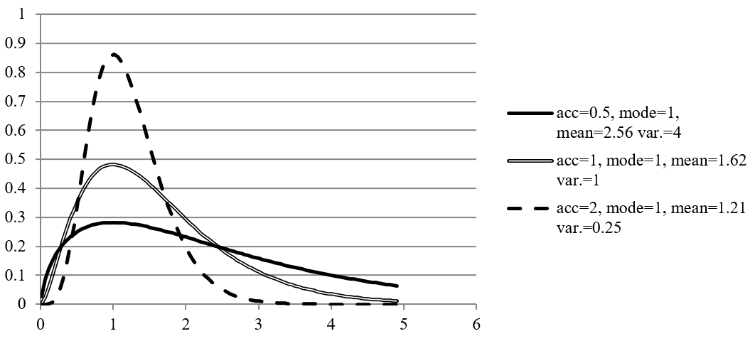
Figure 1: Gamma density graph for mode=1 and various standard deviations. “acc”=“mode/standard deviation”.
Let $i$ denote land use classes in CAPRI definition, whereas l and k are land uses in UNFCCC classification. Let $\text{LU}_{k}$ be total land use after transitions and $\text{LU}_{l}^{\text{initial}}$ be land use before transitions. Furthermore, let $T_{\text{lk}}$ denote the transition of land from use $l$ to use $k$. Noting that it is simpler and fully equivalent to maximize a sum of logged densities than a product of densities, the likelihood maximization problem can be written (with f being the gamma density function)
$${\max_{T_{\text{lk}}}{\log{\prod_{\text{lk}}^{}{f\left( T_{\text{lk}}|\alpha_{\text{lk}},\beta_{\text{lk}} \right)}}}}{= \max_{T_{\text{lk}}}{\sum_{\text{lk}}^{}{\log{f\left( T_{\text{lk}}|\alpha_{\text{lk}},\beta_{\text{lk}} \right)}}}}$$
$$\Rightarrow \max_{T_{\text{lk}}}\sum_{\text{lk}}^{}\left\lbrack \left( \alpha_{\text{lk}} - 1 \right)\log T_{\text{lk}} - \beta_{\text{lk}}T_{\text{lk}} \right\rbrack$$
subject to
$$\text{LU}_{k} - \sum_{l}^{}T_{\text{lk}} = 0 \; \left\lbrack \tau_{k} \right\rbrack$$
$$\text{LU}_{l}^{\text{initial}} - \sum_{k}^{}T_{\text{lk}} = 0\;\left\lbrack \tau_{l}^{\text{initial}} \right\rbrack$$
$$\text{LU}_{k} - \sum_{i}^{}{\text{shar}e_{\text{ki}}\text{LEV}L_{i}} = 0$$
The last equation is needed to convert land use in UNFCCC classification to land use in CAPRI classification, using a fixed linear transformation matrix $\text{shar}e_{\text{ki}}$. This discrepancy between land class accounts will be expanded on in a subsequent section. Forming the Lagrangian function and taking the derivatives with respect to land transitions gives the following first-order optimality conditions:
$$\ \left( \alpha_{\text{lk}} - 1 \right)T_{\text{lk}}^{- 1} - \beta_{\text{lk}} + \tau_{k}^{} + \tau_{l}^{\text{initial}} = 0$$
The parameters $\alpha$ and $\beta$ of the gamma density function were computed by assuming that (i) the observed transitions are the mode of the density, and (ii) the standard deviation equals the mode. Then the parameters are obtained by solving the following quadratic system:
$$\text{mode} = \frac{\alpha - 1}{\beta}$$
$$\text{variance} = \frac{\alpha}{\beta^{2}}$$
Annual transitions via Marcov chain in basic model
The implementation in CAPRI differs from the above general framework in that it explicitly identifies the annual transitions in year t $T_{\text{lk}}^{t}$ from the initial $\text{LU}_{l}^{\text{initial}}$ land use to the final land use $\text{LU}_{k}$. This is necessary to identify the annual carbon effects occurring only in the final year in order to add them to the current GHG emissions, say from mineral fertiliser application in the final simulation year. If the initial year is the base year = 2008 and projection is for 2030, then the carbon effects related to the change from the 2008 $\text{LU}_{l}^{\text{initial}}$ to the final land use $\text{LU}_{k}$ (=$T_{\text{lk}}$in the above notation, without time index) refer to a period of 22 years that cannot reasonably be aggregated with the “running” non-CO2 effects from the final year 2030. Furthermore the historical time series used to determine the mode of the gamma density for the transitions also refer to annual transitions.
Initially the problem to link total to annual transitions has been solved by assuming a linear time path from the initial to the final period, but this was criticised as being an inconsistent time path (by FW). Ultimately the time path has been computed therefore in the supply model in line with a static Markov chain with constant probabilities $P_{\text{lk}}$ such that both land use $\text{LU}_{l}^{t}$ as well as transitions $T_{\text{lk}}^{t}$ in absolute ha require a time index (e_luOverTime in supply_model.gms).
$$\text{LU}_{k}^{t} - \sum_{l}^{}{P_{\text{lk}}\text{LU}_{l}^{t - 1}} = 0\ ,\ t = \{ 1,\ldots s\}$$
Where $\text{LU}_{k}^{s}$ is the final land use in the simulation year s and $\text{LU}_{k}^{0} = \text{LU}_{k}^{\text{iniital}}$ is the initial land use. The transitions in ha in any year may be recovered from previous years land use and the annual (and constant) transition probabilities (e_LUCfromMatrix in supply_model.gms).
$$T_{\text{lk}}^{t} = P_{\text{lk}}*\text{LU}_{l}^{t - 1}$$
The absolute transitions may enter the carbon accounting (ignored here) and if we substitute the last period’s transitions we are back to the condition for consistent land balancing in the final period from above:
$$\text{LU}_{k}^{s} = \sum_{l}^{}{P_{\text{lk}}\text{LU}_{l}^{s - 1}} = \sum_{l}^{}T_{\text{lk}}^{s}$$
When using the transition probabilities in the consistency condition for initial land use we obtain
$$\text{LU}_{l}^{\text{initial}} - \sum_{k}^{}T_{\text{lk}}^{1} = 0$$
$$\Longleftrightarrow \text{LU}_{l}^{\text{initial}} = \sum_{k}^{}{P_{\text{lk}}^{}\text{LU}}_{l}^{\text{iniital}}$$
$$\Leftrightarrow 1 = \sum_{k}^{}P_{\text{lk}}$$
So the simple condition is that probabilities have to add up to one (e_addUpTransMatrix in supply_model.gms).
Annual transitions if SUPREMA is active
As the use of the Marcov-chain approach allows the annual transitions to be explicit model variables that could be used to compute annual carbon effects but leads to computational limitations especially in the market model a new approach was developed under SUPREMA (i.e. if %supremaSup% == on) by re-specifying the total land transitions as average transitions per year times the projection horizon and by considering for the remaining class without land use change (on the diagonal of the land transition matrix) only the annual carbon effects per ha, relevant for the case of gains via forest management.
The new accounting in the CAPRI global supply model may be explained as follows, starting from a calculation of the total GHG effects G over horizon h = t-s from total land transitions Llk and carbon effects per ha for the whole period elk:
$$G = Γ*h = \sum_{i,l}^{}{e_{\text{il}}^{}\text{L}}_{il}^{}$$
Where Γ collects the annual GHG effects that correspond to the total GHG effects divided by the time horizon G / h. These annual effects may be calculated as based on average annual transitions and annual effects for the remaining class as follows:
$$Γ= \sum_{i,l}^{}{e_{\text{il}}^{}\text{L}}_{il}^{}/h = \sum_{i≠l}^{}{e_{\text{il}}^{}\text{Λ}}_{il}^{} + \sum_{i}^{}{ε_{\text{ii}}^{}\text{L}}_{ii}^{} $$
Where Λil = Lil / h is the average land use change per year and εii is the annual carbon effect on a remaining class (relevant might be an annual increase due to growing forests while this will be zero for most effects based on IPCC default assumptions).
Using these average annual transitions for true (off-diagonal) LUC we may compute the final classes as follows:
$$ \text{LU}_{k,t} = \sum_{l}^{}{L_{\text{lk}}^{}\text{}}_{}^{} = \sum_{l≠k}^{}{Λ_{\text{lk}}^{}*h +\text{LU}_{kk}\text{}}_{}^{}$$
While adding up of shares (or probabilities) of LUC from class I to k over all receiving classes k continues to hold as stated above. It should be highlighted that the land use accounting implemented under SUPREMA avoids the need to explicitly trace the annual transitions in the form of a Markov chain and thereby economised on equations and variables.
Outer model – land supply
The outer problem is defined as a maximization of the sum of land rents minus a quadratic cost term, subject to the first order optimality conditions of the inner problem:
$$\max{\sum_{i}^{}{\text{LEV}L_{i}r_{i}} - \sum_{i}^{}{\text{LEV}L_{i}c_{i}} - \frac{1}{2}\sum_{\text{ij}}^{}{\text{LEV}L_{i}D_{\text{ij}}\text{LEV}L_{j}}}$$
subject to,
$$\text{LU}_{k} - \sum_{i}^{}{\text{shar}e_{\text{ki}}\text{LEV}L_{i}} = 0$$
$$\text{LU}_{k} - \sum_{l}^{}T_{\text{lk}} = 0\;\left\lbrack \tau_{k} \right\rbrack$$
$$\text{LU}_{l}^{\text{initial}} - \sum_{k}^{}T_{\text{lk}} = 0\;\left\lbrack \tau_{l}^{\text{initial}} \right\rbrack$$
$$\ \left( \alpha_{\text{lk}} - 1 \right)T_{\text{lk}}^{- 1} - \beta_{\text{lk}} + \tau_{k}^{} + \tau_{l}^{\text{initial}} = 0$$
The parameters of the inner model α and β may be determined as explained in the previous sections. For the outer model, we need to define the parameters c and D. We have a single data point of land use and land rent for each land use class. Since we have, for $N$ land classes, $N + N(N - 1)/2$ parameters, but only $N$ price-quantity pairs (one data point for each land class). This means that without any additional information, we could e.g. calibrate the model exactly by computing the c parameter, but have no information left for defining D. However, we have at our disposal prior estimates of the regional matrices of land supply elasticities that may be used to define prior densities for the elasticity matrix implied jointly by the c and D parameters and the inner problem. Another way of expressing this is that we compute a meta parameter matrix $\mathbf{\eta}\left( \mathbf{c},\mathbf{D},\mathbf{L}\mathbf{U}^{\text{initial}} \right)$ that is a function of the real parameters, and use the prior elasticity matrix as a prior for this meta parameter. If cast in this way, the problem becomes a Bayesian econometric estimation.
There are a few methodological and numerical challenges to overcome. In particular, we need to (i) analytically derive $\mathbf{\eta}\left( \mathbf{c},\mathbf{D},\mathbf{L}\mathbf{U}^{\text{initial}} \right)$, and (ii) ensure that the resulting model has the appropriate curvature to ensure a unique interior solution – anything else would result in a rather useless model. We start by simplifying the problem by observing that all the constraints (the first order conditions of the inner problem) can be replaced with an ordinary land constraint:
$$\sum_{i}^{}{\text{LEV}L_{i}} - \sum_{l}^{}{LU_{l}^{\text{initial}}} = 0$$
Note that the second sum is a constant. This simplification is based on the observation that the land transitions don’t appear in the objective function of the outer problem, so that all solutions to the inner problems are equivalent from the perspective of the outer problem, and that any land use vector that preserves the initial land endowment is a feasible solution to the inner problem.
Next, we formulate the first order condition (FOC) of the modified outer problem to obtain land use as an implicit function of the parameters, $F\left( LEVL,c,D,LU^{\text{initial}},r \right) = 0$. We can then use the implicit function theorem to compute the derivative of land supply $\text{LEV}L_{i}$ with respect to land rent $r_{j}$, which in turn can be used to define the elasticity matrix $\mathbf{\eta}$.
The first order conditions, and the implicit function, become
$$F\left( LEVL,\lambda,c,D,LU^{\text{initial}},r \right) = \begin{bmatrix} \frac{\partial\mathcal{L}}{\partial LEVL_{i}} = & r_{i} - c_{i} - \sum_{j}^{}{D_{\text{ij}}\text{LEV}L_{j}} - \lambda & = 0 \\ \frac{\partial\mathcal{L}}{\partial\lambda} = & \sum_{i}^{}{\text{LEV}L_{i}} - \sum_{l}^{}{LU_{l}^{\text{initial}}} & = 0 \\ \end{bmatrix}$$
In order to apply the implicit function theorem7) we need to differentiate the FOC once w.r.t. the variables $\text{LEV}L_{i}$ and $\lambda$ and once with respect to the parameter of interest, $r_{j}$, invert the former and take the negative of the matrix product. If (currently) irrelevant parameter are omitted, the following matrix of $(N + 1) \times (N + 1)$ is obtained (the “+1” is the uninteresting derivative of total land rent $\lambda$ with respect to individual land class rent $r_{i}$)
$$\left\lbrack \frac{\partial LEVL}{\partial r} \right\rbrack = - \left\lbrack D_{LEVL,\lambda}F(LEVL,\lambda,r) \right\rbrack^{- 1}D_{r}F(LEVL,\lambda,r)$$
$$\begin{bmatrix} \frac{\partial LEVL}{\partial r} \\ \frac{\partial\lambda}{\partial r} \\ \end{bmatrix} = - \begin{bmatrix} \frac{\partial F}{\partial LEVL} & \frac{\partial F}{\partial\lambda} \\ \end{bmatrix}\left\lbrack \frac{\partial F}{\partial r} \right\rbrack$$
Carrying out the differentiation specifically for land rent rj, we obtain:
$$\begin{bmatrix} \frac{\partial LEVL_{i}}{\partial r_{j}} \\ \frac{\partial\lambda}{\partial r_{j}} \\ \end{bmatrix} = - \begin{bmatrix} \left\lbrack {- D}_{\text{ij}} \right\rbrack & - 1 \\ - 1' & 0 \\ \end{bmatrix}^{- 1}\begin{bmatrix} I \\ 0 \\ \end{bmatrix}$$
Discarding the last row of the resulting $(N + 1) \times N$ matrix finally lets us compute the elasticity as
$$\left\lbrack \eta_{\text{ij}} \right\rbrack = \left\lbrack \frac{\partial LEVL_{i}}{\partial r_{j}} \right\rbrack\left\lbrack \frac{r_{j}}{\text{LEV}L_{i}} \right\rbrack$$
In the estimation, we assumed that the prior elasticity matrix is the mode of a density where each entry were independently distributed. Furthermore, the off-diagonal or any diagonal elements with negative priors were normally distributed, whereas the diagonal elements with positive priors (as required for a well-behaved curvature) were gamma distributed. For the standard deviation of elasticities we used either information from the prior estimates or some fall-back assumptions on standard deviations relative to the mode of elasticities. Denoting the prior elasticities with $e_{\text{ij}}$, we solved the following optimization problem, where parameters $\alpha$ and $\beta$ were already estimates as explained in the sections on the inner problem.
$$\max_{\eta,c,D}{\sum_{ij \in normal(i,j)}^{}{- {\frac{1}{s_{\text{ij}}^{2}}\left( \eta_{\text{ij}} - e_{\text{ij}}^{\text{jsa}} \right)}^{2}} + \sum_{ij \in gamma(i,j)}^{}\left\lbrack \left( \alpha_{\text{ij}} - 1 \right)\log\eta_{\text{ij}} - \beta_{\text{ij}}\eta_{\text{ij}} \right\rbrack}$$
subject to
$$\left\lbrack \frac{\partial LEVL_{i}}{\partial r_{j}} \right\rbrack = - \begin{bmatrix} \left\lbrack {- D}_{\text{ij}} \right\rbrack & - 1 \\ - 1' & 0 \\ \end{bmatrix}^{- 1}\begin{bmatrix} I \\ 0 \\ \end{bmatrix}$$
$$\left\lbrack \eta_{\text{ij}} \right\rbrack = \left\lbrack \frac{\partial LEVL_{i}}{\partial r_{j}} \right\rbrack\left\lbrack \frac{r_{j}}{\text{LEV}L_{i}} \right\rbrack$$
$$\begin{matrix} & r_{i} - c_{i} - \sum_{j}^{}{D_{\text{ij}}\text{LEV}L_{j}} - \lambda & = 0 \\ & \sum_{i}^{}{\text{LEV}L_{i}} - \sum_{l}^{}{LU_{l}^{\text{initial}}} & = 0 \\ \end{matrix}$$
and the curvature constraint using a stricter variant of the Cholesky factorization
$$D_{\text{ij}}\left( 1 - \delta I_{\text{ij}} \right) = \sum_{k}^{}{U_{\text{ki}}U_{\text{kj}}}$$
where $\delta$ is a small positive number and $I_{\text{ij}}$ entries of the identity matrix such that the factor $(1 - \delta I_{\text{ij}})$ shrinks the diagonal of the D-matrix, ensuring strict positive definiteness instead of semi-definiteness. We used $\delta = 0.05$. Furthermore, the Lagrange multiplier of the total land constraint, $\lambda$, was fixed at the weighted average of the rents $r_{i}$, i.e. $\lambda = \frac{\sum_{i}^{}{\text{LEV}L_{i}r_{i}}}{\sum_{i}^{}{\text{LEV}L_{i}}}$. Without the latter assumption, the parameters c and D are not uniquely identified.
Prior elasticities and area mappings
The empirical evidence obtained in the TRUSTEE project applied to prior elasticities for land categories based on Corine Land Cover (CLC) data. These categories are also covered in the CAPRI database based on various sources (see the database section in the CAPRI documentation):
The introduction has mentioned already three systems of area categories that need to be distinguished. The first one is the set of area aggregates with good coverage in statistics that has been investigated recently by JS Ay (2016), in the following “JSA”:
$$\text{LEVL} = \left\{ \text{ARAC},\ \text{FRUN},\ \text{GRAS},\ \text{FORE},\ \text{ARTIF},\text{OLND} \right\}$$
Where
ARAC = arable crops
FRUN = perennial crops
GRAS = permanent grassland
FORE = forest
ARTIF = artificial surfaces (settlements, traffic or industrial)
OLND = other land
The above categories are matching reasonably well with the definitions in JSA. A mismatch exists in the classification of paddy (part of ARAC in CAPRI but in the perennial group in JSA) and terrestrial wetlands (part of OLND in CAPRI and a separate category in JSA). Inland waters are considered exogenous in CAPRI and hence not included in the above set LEVL.
For carbon accounting we need to identify the six LU classes from IPCC recommendations and official UNFCCC reporting:
$$LU = \left\{ \text{CROP},\ \text{GRS}\text{LND},\ \text{FORE},\ \text{ARTIF},WETLND,RESLND \right\}$$
which is typically indexed below with “l” or “k” ∈ LU and where
CROP = crop land (= sum of arable crops and perennial crops)
GRSLND = grassland in IPCC definition (includes some shrub land and other “nature land”, hence GRSLND>GRAS)
WETLND = wetland (includes inland waters but also terrestrial wetlands)
RESLND = residual land is that part of OLND not allocated to grassland or wetland, hence RESLND<OLND
FORE = forest
ARTIF = artificial surfaces
In the CAPRI database, in particular for its technical base year, we have estimated an allocation of other land OLND into its components attributable to the UNFCCC classes GRSLND,WETLND, and RESLND:
$$\text{OLND}^{0} = {\text{OLND}G}^{0} + {\text{OLND}W}^{0} + {\text{OLND}R}^{0}$$
Lacking better options to make the link between sets LEVL (activity level aggregates) and LU (UNFCCC classes, technically in CAPRI code: set “LUclass”) we will assume that these shares are fixed and may estimate the “mixed” LU areas from activity level aggregates as follows
| GRSLND | = | GRAS + OLND · OLNDG0/OLND0 |
|---|---|---|
| WETLND | = | INLW + OLND · OLNDW0/OLND0 |
| RESLND | = | OLND · OLNDR0/OLND0 |
which means that the mapping from set LEVL to set LU only uses some fixed shares of LEVL areas that are mapped to a certain LU:
$$LU_k=\sum_i{\text{share}_{\text{i,k}}\text{LEVL}_i}$$
where 0 ≤ sharei,k ≤ 1.
Technical implementation
The key equations corresponding to the approach explained above are collected in file supply_model.gms or the included files supply/declare_calibration_models_for_luc.gms and supply/declare_calibration_models_for_land_supply.gms. The declarations of parameters, variables, equations, models and even some sets only used in the calibration given in these files are included by the “supply_model.gms” only if “BASELINE==ON” or if it was a CAPREG base year task that was carried out. Loading of priors, initialisation of parameters and variables for the calibration as well as the organisation of solve attempts are handled in new sections of file “cal_land_nests.gms”, in turn called by the gams file “prep_cal.gms”. This implies that the land supply and land use change calibrations were inserted before the ordinary calibration of the supply models.
SupremaSup should be active together with trustee_land to have smoother adjustments which may be set via the CAPRI GUI. In order to store the results of the calibration in a compact way that is compatible with the existing code, the existing parameter files “pmppar_XX.gdx” was used. The parameters of the land supply functions, called “c” and “D” above, were stored on two parameters “p_pmpCnstLandTypes” and “p_pmpQuadLandTypes”. As a new symbol (p_pmpCnstLandTypes) is introduced in an existing file, the first run of CAPRI after setting %trustee_land%==on may give errors if the file exists already but has been used with the previous land supply specification before. In this case it helps to delete or rename the old pmppar files.
At this point, it should also be explained that rents for non-agricultural land types were entirely based on assumptions (a certain ratio to agricultural rents). As there were no plans to run scenarios with modified non-agricultural rents, these land rents r used in calibration for those land types were subtracted from the “c-paramter”, so that it is implicitly stored in p_pmpCnstLandTypes and enters the objective function through the PMP terms. This requires changes if the rents shall be modified or if non-agricultural production shall be included in some simplified form.
Furthermore, the class Inland Waters (INLW) was given a special treatment: it is supposed to be entirely exogenous. For this purpose the special acronym “exogenousLandSupply” was introduced, and stored on the p_pmpCnstLandTypes and used to trigger an equation “e_exogenousLand “ in the supply model setting the variable to a constant. In that way, the fixity of INLW (or any land type, should it happen) is stored in the pmp terms and cannot be “forgotten”.
More detailed explanations on the technical implementation are covered elsewhere, for example in the “Training material” included in the EcAMPA-4 deliverable D5.
Concerning the improvements made under SUPREMA from a technical perspective, the changes are merged to the trunk. The approach is controlled by globals in capmod\set_global_variables.gms. If the global variable %supremaSup% == on, the yearly transition rate p_lucAnnualFac_sup is calculated. If it is %supremaSup% == off, the old approach using the Marcov chain is used with the respective variable v_luYearly. The FOC-approach to calculate LUC as described above is standard and independent from if the global variable supremaSup is on or off.
Emission Equations
Under EcAMPA 3 and partly in earlier projects (inter alia EcAMPA 2) new modelling outputs have been developed for indicators without matching reporting infrastructure helping users to organise the additional information. This applied for example to
1) Additional CAPRI results on land use results related to the complete area coverage, mappings to UNFCCC area categories and their transitions;
2) The carbon effects linked to these land transitions.
Furthermore, additional non-CO2 and CO2 related mitigation measures had been included under EcAMPA 3.
The scenarios including the emission equations are only run if %ghgabatement% == on, otherwise emissions are only calculated and not simulated.
The following emission equations have been implemented:
| Code | Description |
|---|---|
| GWPA | Agricultural emissions |
| CH4ENT | Methane emissions from enteric fermentation |
| CH4MAN | Methane emissions from manure management |
| CH4RIC | Methane emissions from rice production |
| N2OMAN | Direct nitrous oxide emissions stemming from manure management (only housing and storage) |
| N2OAPP | Direct nitrous oxide emissions stemming from manure application on soils except grazings per animal activity |
| N2OGRA | Direct nitrous oxide emissions stemming from manure managment on grazings |
| N2OSYN | Direct nitrous oxide emissions from anorganic fertilizer application |
| N2OCRO | Direct nitrous oxide emissions from crop residues |
| N2OAMM | Indirect nitrous oxide emissions from ammonia volatilisation |
| N2OLEA | Indirect nitrous oxide emissions from leaching |
| N2OHIS | Direct nitrous oxide emissions from cultivation of histosols |
| GLUC | Emissions related to indirect land use changes |
| CO2BIO | Carbon dioxide emissions from land use change due to losses of carbon in biomass and litter |
| CO2SOI | Carbon dioxide emissions from land use change due to soil carbon losses |
| CO2HIS CH4HIS | Carbon dioxide emissions from the cultivation of histosols Methane emissions from cultivation of histosols |
| CO2LIM CO2BUR | Carbon dioxide emissions from limestone and dolomit Carbon dioxide emissions from burning |
| CH4BUR | Methane emissions from burning |
| N2OBUR | Nitrous oxide emissions from burning |
| N2OSOI | N2O emissions from land use change due to soil carbon losses |
| GPRD | Emissions related to the production of non-agricultural inputs to agriculture |
| N2OPRD | Nitrous oxide emissions during fertilizer production |
| O2PRD | Carbon Dioxide emissions during fertilizer production |
1)
A more complete presentation is given in https://ec.europa.eu/jrc/en/publication/eur-scientific-and-technical-research-reports/extension-capri-model-irrigation-sub-module.
2)
These are most completely included in the “trunk” version of the CAPRI system. For details, see, for example, http://publications.jrc.ec.europa.eu/repository/bitstream/JRC101396/jrc101396_ecampa2_final_report.pdf.
3)
These are most completely included in the “trunk” version of the CAPRI system but developments are still ongoing.
7)
Recall that the implicit function theorem states that if F(x,p) = 0, then dx/dp = -[dF/dx]-1[dF/dp]
module_for_agricultural_supply_at_regional_level.txt · Last modified: 2023/09/08 12:11 by massfeller