The idea behind the decomposition is to analyze which factors drive the change in yields and income indicators using growth rates. Take for example the market income of cereals per ha at EU level. Its change in a simulation against the baseline depends on the change in prices and the change in yields. The change in yields in turns depends on the effect of the yield elasticity, the change in the shares of low and high technology variants, the change in the regional shares and, in weights of low and high yielding regions. And finally, the share of high and low yielding cereals such as soft what and rye in the total aggregate might change. When interpreting the results, it is often useful to understand the contribution of the different factors.

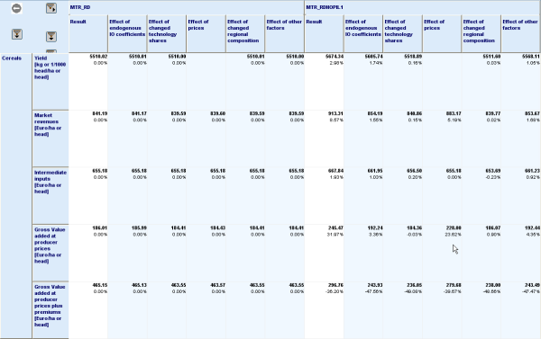
The screenshot below shows an example. All results shown are always expressed in the absolute value and the units used in the result set.

The columns are defined as follows:

• Result: Final result from the simulation – in the example below, average EU27 cereals yields increase by 8.57%.
• Effect of endogenous IO coefficients: Result calculated by using the final IO coefficients, but keeping all other factors (technology shares, prices, regional weights, activity levels) at trend levels – in the example below, market revenues per ha would have gone up by 1.55% if only the yields had adjusted.
• Effect of technology shares: Result calculated by only updating the technology shares, but keeping all other factors (IO coefficients, prices, regional weights, activity levels) at trend levels – in the example below, intermediate input costs would have increased by 0.2% of only the share of low and high yielding variants had changed.
• Effect of prices: Result calculated by only updating the prices shares, but keeping all other factors (IO coefficients, technology shares, regional weights, activity levels) at trend levels – in the example below, the Gross Value Added at producer prices would have increased by 23.62% if only the input and output prices had changed.
• Effect of regional composition: Result calculated by only updating the activity levels shares, but keeping all other factors (IO coefficients, technology shares, activity levels) at trend levels
• Effect of other factors: Difference between the start values and result, after all other effects above had been accounted for. Comprises the multiplicative cross-effects of the different effects, the effect of changed premiums in the case of the MGVA, and of change in the activity aggregate composition.

Figure 39: Illustrative scenario comparison for the yield and income indicator decomposition

Source: CAPRI modelling system Note: The code is implemented in „reports\yield_change_decomp”. The table can be found in the GUI under “farm ⇒ yield decomposition”.

It should be mentioned that the coding does not use information about potential changes of the premiums paid in scenario against the baseline, so that the results shown for the modified Gross Value Added should mainly show the different percentage changes on income once the level effect of the premiums is considered. The coding also stems from the time before climate related yield shock sceanrios or endogenous mitigation modelling. As the yield decomposition probably has not been regularly checked in this kind of scenarios, it is possible that some changes implemented in the CAPRI supply models need to be transferred to this reporting code to give reliable results in all kind of scenarios.